Gaussian Cloud · Part I
Recursive simulation, conditional errors and Section 6 cost bookkeeping.
Main paper results remain open in Lean. Verified building blocks are listed separately below.
Suggested reading order
- Start with the main theorem to see the accuracy and expected-query destination.
- Read Lemma 6.1 to understand why the adaptive request forest has controlled size before the global cap.
- Read Lemma 6.3 beside the bookkeeping ledger: each conditional replacement contributes one delta_t, while the global cap contributes epsilon_cap exactly once.
Paper, notation and source conventions
High-accuracy simulation of Picard HMC, part I: Gaussian cloud correction
Source: 2609.38710v1. Pinned source version
- The source assumes the normalized target \(\pi\) satisfies \(\operatorname{KL}(\mu\Vert\pi)\le(\kappa/2)I(\mu\Vert\pi)\) for every probability measure \(\mu\) with smooth density, with \(\kappa\ge1\). This is an LSI assumption, not a pointwise strong-convexity hypothesis.
- The supplied reference point satisfies \(\|\nabla V(x_{\mathrm{ref}})\|\le\sqrt{d/\kappa}\). No warm-start law is assumed.
- The strongly log-concave specialization follows only after rescaling the smoothness and LSI constants; the general source theorem is stated under one-smoothness plus LSI.
- Expected gradient queries include the paper's recursive Gaussian-cloud corrections, implemented RGO calls and cap/fallback accounting. They are not a worst-case runtime bound.
1. Main statements
RED · source theorem known · local proof open
Main high-accuracy sampling guarantee
Source: 2609.38710v1. Theorem 1.1; equations (1.1)–(1.2)
Open this theorem in the interactive research workspace
Statement
For the paper's sampler and parameter choices, a one-smooth target satisfying the displayed logarithmic Sobolev inequality can be sampled to total-variation error \(\varepsilon\) with the stated expected number of gradient queries, without a warm-start assumption.
- \(d\ge1\); V is \(C^2\) on \(\mathbb R^d\) and \(\nabla V\) is 1-Lipschitz; \(\pi\) is the normalized law proportional to \(e^{-V}\).
- \(\pi\) satisfies \(\operatorname{KL}(\mu\Vert\pi)\le\kappa/2\) times the relative Fisher information for every probability measure \(\mu\) with smooth density, with \(\kappa\ge1\).
- A supplied reference point \(x_{\mathrm{ref}}\) satisfies \(\|\nabla V(x_{\mathrm{ref}})\|\le\sqrt{d/\kappa}\).
- \(0<\varepsilon\le1/4\); use the source Gaussian-cloud sampler, proximal wrapper and exact parameter schedule rather than an arbitrary Picard discretization.
Lean statement — not formalized yet
A future declaration must bind the probability laws, normalization, regularity, source algorithm and oracle model explicitly. The formula is a source theorem contract, not Lean code.
No corresponding ASTIS declaration is asserted. Search locations below are candidates, not established dependencies or copied library proofs.
Proof architecture and calculations · 4 steps
This is a source-linked proof route, not a complete reconstruction of all cited lemmas. The dependencies below remain separate formalization tasks.
Represent dependent Picard evaluations by Gaussian clouds
\[X_i^{[k]}=\bar X_i^{[k]}+\sqrt{\eta}\,G_i^{[k]}\]The cloud representation exposes independent Gaussian blocks while preserving the shared dependence needed by Picard iteration. Fluctuation and mean corrections are separate FORS gadgets; independence may not be invented between recursively shared blocks.
Source: 2609.38710v1. Sections 3.1 and 4–5
Track or question this step in Live Formalization
Lean step — not formalized yet
This mathematical step is still open in Lean. The future declaration must expose exactly the objects and side conditions named above; no source-cited wrapper is counted as a proof.
No corresponding ASTIS declaration is asserted. Search locations below are candidates, not established dependencies or copied library proofs.
Assemble a finite adaptive computation
\[A_{v+1}=A_v-1+\zeta_{v+1},\qquad T=\inf\{v:A_v=0\}\]Mandatory predecessor chains are contracted into vertices and optional nested requests become children. Lemmas 6.1 and 6.2 control vertices and attached RGO queries before the deterministic global cap is imposed.
Source: 2609.38710v1. Section 6.1; Lemmas 6.1–6.2
Track or question this step in Live Formalization
Lean step — not formalized yet
This mathematical step is still open in Lean. The future declaration must expose exactly the objects and side conditions named above; no source-cited wrapper is counted as a proof.
No corresponding ASTIS declaration is asserted. Search locations below are candidates, not established dependencies or copied library proofs.
Telescope every implementation error
\[\mathsf{TV}(\operatorname{Law}(\widehat X),\operatorname{Law}(X))\le\sum_{t=1}^{T_{\max}}\delta_t+\varepsilon_{\rm cap}\]Dummy filling converts early termination into a common fixed slot space. Hybrids replace one conditional kernel at a time under the ideal history; the cap failure is added only after comparing capped and uncapped ideal algorithms.
Source: 2609.38710v1. Lemma 6.3
Track or question this step in Live Formalization
Lean step — not formalized yet
This mathematical step is still open in Lean. The future declaration must expose exactly the objects and side conditions named above; no source-cited wrapper is counted as a proof.
No corresponding ASTIS declaration is asserted. Search locations below are candidates, not established dependencies or copied library proofs.
Insert the Section 6 budgets into the cloud sampler
\[\mathbb E Q_{\nabla}\le C\mathfrak L^{11/2}(d+\mathfrak L)^{1/5}\]Theorem 6.4 fixes h, smoothing levels, Picard depth, phase count, local correction budgets and RGO accuracies. The proximal wrapper then restores general condition number \(\kappa\) and produces Theorem 1.1.
Source: 2609.38710v1. Theorem 6.4; proof of Theorem 1.1
Track or question this step in Live Formalization
Lean step — not formalized yet
This mathematical step is still open in Lean. The future declaration must expose exactly the objects and side conditions named above; no source-cited wrapper is counted as a proof.
No corresponding ASTIS declaration is asserted. Search locations below are candidates, not established dependencies or copied library proofs.
Lean proof — not formalized yet
Formalization will first match the named technology interfaces, then assemble this source theorem. No placeholder proof or source-cited wrapper has been added.
No corresponding ASTIS declaration is asserted. Search locations below are candidates, not established dependencies or copied library proofs.
Strict boundary
No local Lean theorem yet proves the sampler, the adaptive forest, or the complexity bound. The big-O hides only universal constants specified by the source parameter choices; it is not a license to omit \(\kappa\), dimension, precision, cap or initialization dependencies.
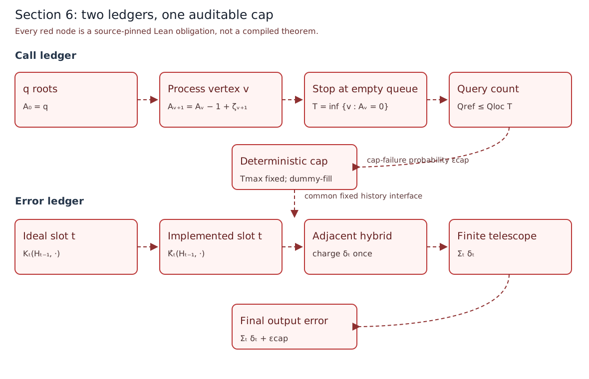
Section 6: follow the recursive calls and accumulated errors
SOURCE-PINNED LEDGER · Lean formalization open
Section 6 recursive-call and accumulated-error ledger
The paper's adaptive sampler is easiest to audit as two coupled ledgers. The call ledger counts a breadth-first request forest. The error ledger compares ideal and implemented conditional kernels one slot at a time. They meet at the deterministic cap \(T_{\max}\); they must not be collapsed into one informal union bound.
| Symbol | Meaning | Definition or update | Why it is tracked |
|---|---|---|---|
\[q\] | Initial root requests | \[A_0=q\] | Starts the request forest; it is not the final query count. |
\[A_v\] | Pending requests after v vertices | \[A_{v+1}=A_v-1+\zeta_{v+1}\] | Queue state used to define termination. |
\[\zeta_{v+1}\] | Children revealed by the next processed vertex | \[\mathbb E[e^{s\zeta_{v+1}}\mid\mathcal F_v]\le e^{\lambda(e^{ms}-1)}\] | Controls both drift and the tail of the adaptive tree. |
\[T\] | First v with \(A_v=0\) | \[\mathbb ET\le4q/3,\quad\mathbb P\{T>C(q+mu)\}\le e^{-u}\] | Counts contracted vertices before the global cap. |
\[Q_{\rm loc}\] | Local reference-query cap per vertex | \[Q_{\rm loc}=C\mathfrak L^2\] | Turns a vertex-count bound into a reference-query bound. |
\[T_{\max}\] | Deterministic number of recorded call slots | \[T_{\max}=\lceil C(N+\mathfrak L^3)\mathfrak L^2\rceil\] | Makes the adaptive execution a fixed-length history after dummy filling. |
\[\delta_t\] | Mean TV error at slot t under ideal capped history | \[\mathbb E\,\mathsf{TV}(K_t(H_{t-1},\cdot),\widehat K_t(H_{t-1},\cdot))\] | Charged once by the adjacent-hybrid comparison. |
\[\varepsilon_{\rm cap}\] | Ideal probability of exceeding the global cap | \[\mathbb P\{T>T_{\max}\}\le\varepsilon_{\rm cap}\] | Charged once when capped ideal output is compared with uncapped ideal output. |
Where each error enters
Potential request schedule
Input. FORS attempts and nested cloud/RGO requests
Output. A dominating adaptive forest
Ledger charge. No accuracy error; this is a counting enlargement.
Local and global caps
Input. Tree-size and per-vertex query tails
Output. A finite record of at most \(T_{\max}\) slots
Ledger charge. Only the ideal global-cap failure contributes \(\varepsilon_{\mathrm{cap}}\) in Lemma 6.3.
Slot t replacement
Input. Same ideal history \(H_{t-1}\)
Output. Replace K_t by Khat_t
Ledger charge. \(\delta_t\); later adaptive behavior is handled by data processing.
Hybrid telescope
Input. \(T_{\max}\) adjacent algorithm pairs
Output. Implemented capped law versus ideal capped law
Ledger charge. Sum from t=1 to \(T_{\max}\) of \(\delta_t\).
Final cap comparison
Input. Ideal capped and ideal uncapped outputs
Output. Actual target algorithm comparison
Ledger charge. Add \(\varepsilon_{\mathrm{cap}}\), giving sum \(\delta_t\) + \(\varepsilon_{\mathrm{cap}}\).
Lean ledger interface — not formalized yet
The first Lean packet will formalize the fixed finite dummy-filled history and adjacent-hybrid TV telescope. Adaptive-tree tails, concrete cloud kernels and final parameter substitution stay separate.
No corresponding ASTIS declaration is asserted. Search locations below are candidates, not established dependencies or copied library proofs.
Strict boundary
This ledger does not prove the conditional-kernel bounds, the adaptive-tree moment estimate, measurability of histories, or the paper's final parameter substitution. Each remains a separate theorem obligation. Dummy filling is part of the mathematical interface, not presentation-only padding.
Further source statements · 2
RED · source theorem known · local proof open
Size and query count of a capped adaptive tree
Source: 2609.38710v1. Section 6.1, Lemma 6.1, equations (6.1)–(6.2)
Open this theorem in the interactive research workspace
Statement
A breadth-first request queue with conditionally sub-Poisson child counts and mean offspring at most one quarter has expected total size at most four thirds of its root count and a subexponential upper tail. A deterministic local query cap multiplies the vertex bound.
- \(q\ge1\) roots; \(A_0=q\) and, while \(A_v>0\), \(A_{v+1}=A_v-1+\zeta_{v+1}\) with \(\zeta_{v+1}\) a nonnegative integer adapted to the exploration filtration.
- Deterministic \(m\ge1\) and \(\lambda\ge0\) satisfy \(\mathbb E[e^{s\zeta_{v+1}}\mid\mathcal F_v]\le e^{\lambda(e^{ms}-1)}\) on {\(A_v>0\)}, for every \(0\le s\le1/m\).
- \(m\lambda\le1/4\); T is the first v with \(A_v=0\). The local reference-query count per processed vertex is at most \(Q_{\mathrm{loc}}\).
Lean statement — not formalized yet
A future declaration must bind the probability laws, normalization, regularity, source algorithm and oracle model explicitly. The formula is a source theorem contract, not Lean code.
No corresponding ASTIS declaration is asserted. Search locations below are candidates, not established dependencies or copied library proofs.
Proof architecture and calculations · 3 steps
This is a source-linked proof route, not a complete reconstruction of all cited lemmas. The dependencies below remain separate formalization tasks.
Differentiate the conditional MGF at zero
\[\mathbb E[\zeta_{v+1}\mid\mathcal F_v]\le m\lambda\le\tfrac14\]This supplies negative queue drift while the process is alive. Lean must state the conditional-expectation version and the stopped extension after the queue empties.
Source: 2609.38710v1. Lemma 6.1 proof, expectation estimate
Track or question this step in Live Formalization
Lean step — not formalized yet
This mathematical step is still open in Lean. The future declaration must expose exactly the objects and side conditions named above; no source-cited wrapper is counted as a proof.
No corresponding ASTIS declaration is asserted. Search locations below are candidates, not established dependencies or copied library proofs.
Sum the stopped drift
\[\mathbb E A_{n\wedge T}\le q-\tfrac34\,\mathbb E(n\wedge T)\]Nonnegativity of the queue yields a uniform bound on the stopped exploration time; monotone convergence then gives the expectation bound for T.
Source: 2609.38710v1. Lemma 6.1 proof, expected size
Track or question this step in Live Formalization
Lean step — not formalized yet
This mathematical step is still open in Lean. The future declaration must expose exactly the objects and side conditions named above; no source-cited wrapper is counted as a proof.
No corresponding ASTIS declaration is asserted. Search locations below are candidates, not established dependencies or copied library proofs.
Build the exponential supermartingale
\[\mathbb P\{T>C(q+mu)\}\le e^{-u}\]The conditional MGF assumption controls the stopped queue and gives the tail with a universal constant C. This step must track the permitted range \(0\le s\le1/m\) rather than optimize over an illegal exponent.
Source: 2609.38710v1. Lemma 6.1 proof, tail bound
Track or question this step in Live Formalization
Lean step — not formalized yet
This mathematical step is still open in Lean. The future declaration must expose exactly the objects and side conditions named above; no source-cited wrapper is counted as a proof.
No corresponding ASTIS declaration is asserted. Search locations below are candidates, not established dependencies or copied library proofs.
Lean proof — not formalized yet
Formalization will first match the named technology interfaces, then assemble this source theorem. No placeholder proof or source-cited wrapper has been added.
No corresponding ASTIS declaration is asserted. Search locations below are candidates, not established dependencies or copied library proofs.
Strict boundary
This lemma counts a dominating potential request tree. It does not prove that any particular FORS/cloud implementation satisfies the MGF premise, and it does not include RGO-internal query counts except through the separate attachment analysis.
RED · source theorem known · local proof open
Adaptive conditional-kernel TV error telescope
Source: 2609.38710v1. Section 6.1, Lemma 6.3
Open this theorem in the interactive research workspace
Statement
For ideal and implemented adaptive algorithms stopped at the same deterministic number of slots, the output-law error is at most the sum of the mean conditional replacement errors evaluated along the ideal capped histories, plus the probability that the uncapped ideal algorithm exceeds the cap.
- For each slot \(1\le t\le T_{\max}\), \(K_t(H,\cdot)\) and \(\widehat K_t(H,\cdot)\) are measurable probability kernels on a common history/output interface.
- Both capped algorithms use the same deterministic \(T_{\max}\) and append a measurable dummy symbol after termination.
- The uncapped ideal algorithm exceeds \(T_{\max}\) with probability at most \(\varepsilon_{\mathrm{cap}}\).
- \(H_{t-1}\) is the ideal capped history and \(\delta_t\) is the expectation of \(\operatorname{TV}(K_t(H_{t-1},\cdot),\widehat K_t(H_{t-1},\cdot))\).
Lean statement — not formalized yet
A future declaration must bind the probability laws, normalization, regularity, source algorithm and oracle model explicitly. The formula is a source theorem contract, not Lean code.
No corresponding ASTIS declaration is asserted. Search locations below are candidates, not established dependencies or copied library proofs.
Proof architecture and calculations · 5 steps
This is a source-linked proof route, not a complete reconstruction of all cited lemmas. The dependencies below remain separate formalization tasks.
Freeze a common finite history space
\[H=(Y_1,\ldots,Y_{T_{\max}}),\qquad Y_t=\dagger\text{ after termination}\]Dummy filling makes every adaptive run a fixed-length record. This is what permits the t-th conditional rule to be compared without pretending that both algorithms made the same random number of calls.
Source: 2609.38710v1. Lemma 6.3, setup
Track or question this step in Live Formalization
Lean step — not formalized yet
This mathematical step is still open in Lean. The future declaration must expose exactly the objects and side conditions named above; no source-cited wrapper is counted as a proof.
No corresponding ASTIS declaration is asserted. Search locations below are candidates, not established dependencies or copied library proofs.
Define adjacent hybrids
\[\mathcal A^{(t)}=(K_1,\ldots,K_t,\widehat K_{t+1},\ldots,\widehat K_{T_{\max}})\]Consecutive hybrids share the ideal history distribution through slot t-1. Therefore the only new discrepancy is the conditional kernel at slot t, averaged under precisely that ideal history.
Source: 2609.38710v1. Lemma 6.3 proof
Track or question this step in Live Formalization
Lean step — not formalized yet
This mathematical step is still open in Lean. The future declaration must expose exactly the objects and side conditions named above; no source-cited wrapper is counted as a proof.
No corresponding ASTIS declaration is asserted. Search locations below are candidates, not established dependencies or copied library proofs.
Use data processing for the adaptive suffix
\[\mathsf{TV}(\operatorname{Law}(\mathcal A^{(t)}),\operatorname{Law}(\mathcal A^{(t-1)}))\le\delta_t\]All later calls may depend on the replaced output, but they form one common measurable downstream kernel for this adjacent pair. Data processing absorbs that adaptive continuation.
Source: 2609.38710v1. Lemma 6.3 proof
Track or question this step in Live Formalization
Lean support — compiled reusable edge
The reusable mean conditional-error and common-suffix edges compile. Constructing the paper's dummy-filled history and identifying its slot law remain open.
AutoSamplingTheory.TechnicalLemmas.Probability.KernelHybridTelescope.abs_real_comp_sub_le_integral_eventBoundAutoSamplingTheory.TechnicalLemmas.Probability.KernelHybridTelescope.abs_real_comp_commonSuffix_sub_le_integral_eventBound
Read the statement, mathematical proof and folded Lean source below ↓
Telescope the capped adjacent hybrids
\[\mathsf{TV}(P_{T_{\max}},P_0)\le\sum_{t=1}^{T_{\max}}\delta_t\]Apply the triangle inequality to the fixed finite list of hybrid event probabilities. Every slot budget is charged once with unit coefficient.
Source: 2609.38710v1. Lemma 6.3 proof
Track or question this step in Live Formalization
Lean support — compiled reusable edge
The finite real telescope compiles. Its application still needs the source-specific hybrid laws and adjacent bounds.
AutoSamplingTheory.TechnicalLemmas.Probability.KernelHybridTelescope.abs_sub_zero_le_sum_range_of_adjacent
Read the statement, mathematical proof and folded Lean source below ↓
Add cap failure once
\[\mathsf{TV}(\widehat P,P)\le\mathsf{TV}(\widehat P,P_{\rm capped})+\varepsilon_{\rm cap}\]A final coupling or event comparison handles ideal capped versus ideal uncapped output. This is a separate proof edge, so the cap term is not repeated at every slot.
Source: 2609.38710v1. Lemma 6.3 proof
Track or question this step in Live Formalization
Lean step — not formalized yet
This mathematical step is still open in Lean. The future declaration must expose exactly the objects and side conditions named above; no source-cited wrapper is counted as a proof.
No corresponding ASTIS declaration is asserted. Search locations below are candidates, not established dependencies or copied library proofs.
Lean proof — not formalized yet
Formalization will first match the named technology interfaces, then assemble this source theorem. No placeholder proof or source-cited wrapper has been added.
No corresponding ASTIS declaration is asserted. Search locations below are candidates, not established dependencies or copied library proofs.
Strict boundary
The mean conditional-event integral, common-suffix contraction and finite real telescope now compile as reusable Lean edges. The exact dummy-filled history kernel, source-specific \(\delta_t\) identification and measurability, and capped/uncapped comparison remain separate red obligations; therefore Lemma 6.3 itself is not yet formalized. Uniform \(\varepsilon\) is only a corollary after those adapters.
3. What has been verified?
3 source-mapped declarations; 3 independently reviewed. These are building blocks, not completed paper results.
Browse statements and their mathematical proofs
Adaptive conditional-kernel hybrid telescope
- Average a history-dependent one-call kernel error
- Later adaptive computation cannot amplify one replaced call
- Finite adjacent hybrid errors add
Read full statement and proof →
Source assumptions, verification evidence and optional Lean are beside the proof on that page.