State preparation · Exact Hermite target; polynomial-gate Bernstein–MPS construction; finite export evidence remains separate
Hermite-smoothed initial states
Prepare the sampled smooth auxiliary initial state used in Schrödingerisation, for any Hermite order k. Load function values as amplitudes and account for the preparation circuit itself.
Source paper · general Hermite initial-state family with an ASPBE preparation circuit
Where this example comes from
Schrödingerisation based computationally stable algorithms for ill-posed problems in partial differential equations
Shi Jin, Nana Liu, Chuwen Ma · 2024
Source anchor. Jin–Liu–Ma Sec. 4.3, Eqs. (4.31)–(4.32); cubic example Eq. (6.1)
Sec. 4.3 Eq. (4.31) Eq. (4.32) Eq. (6.1)
What the paper says. The negative half-axis is extended by a degree at most \(2k+1\) Hermite polynomial on [-1,0], matching derivatives through order \(k\) at both endpoints; the positive half-axis remains exp(-p).
What ASPBE does here. ASPBE proves the explicit coefficients, global C^k smoothness and a deterministic primitive rotation circuit for the normalized sampled state. The paper's PDE recovery, Sobolev and convergence results are not claimed as Lean theorems by this case. The C2 sentence after Eq. (6.1) is not adopted: its displayed cubic is C1 at the splice points.
Core insight · start from the mathematical object
Why an exponentially long state can still have a short preparation rule
The state has one amplitude for every grid point, but those amplitudes are not independent data. They all come from the same three-piece Hermite profile. The construction keeps that functional structure while reading the binary address, so the circuit carries only a small working state whose dimension depends on the smoothing order k.
What the reference method actually stores
“Amplitude list” and “mass tree” are concrete objects, not jargon
The reference construction is easiest to understand if we name the two objects that make it generic.
Define this first
Explicit amplitude list
This is what we mean by a sample table: write down all N function values as if they were unrelated input data. It is correct, but it immediately forgets that every entry came from one simple function.
Define this first
Binary mass tree
This is the reference preparation tree: each prefix stores the probability mass under that prefix, and its two child masses determine the next controlled rotation. The tree is transparent, but the number of prefixes grows with the number of samples.
What is special about this family?
The samples come from one short piecewise function
Before discussing MPS, bond dimension or compilation, keep the source formula visible:
1 · keep the source function
Do not turn the Hermite profile into unrelated samples
The left tail, polynomial bridge and right tail each have a finite description. The proof keeps those descriptions alive instead of expanding them into N separate numbers.
2 · read one address bit
A binary digit only chooses the next dyadic half-interval
Reading the address most-significant-bit first is an interval walk. We only need to update enough information to evaluate the same source function on the chosen child interval.
3 · update small analytic memory
Tails need scalars; the polynomial needs Bernstein coefficients
The exponential pieces factor over address bits. On the polynomial piece, exact de Casteljau subdivision maps one short Bernstein coefficient vector to the left or right child vector. Boundary bookkeeping plus the two tails gives total width D=2k+6.
4 · recognize a tensor train
The bit-by-bit finite-state rule is exactly an MPS/TT factorization
The long amplitude vector is represented by n_p local tensors coupled through a D-dimensional bond. The bond is working memory, not another copy of the amplitude table.
5 · compile the bond
Canonicalize locally, complete isometries, then emit elementary gates
Small Gram contractions give the norm; thin LQ makes the chain locally norm preserving; only reachable columns are completed to real unitaries and decomposed into rotations. The bond qubits return to zero.
The matrices are local updates selected by the address bits. The important number is the internal width \(D=2k+6\), not the number \(2^{n_p}\) of output amplitudes.
Mathematical cross-pollination
Each field supplies one indispensable interface
The proof is not “use MPS” as a black box. It changes representation four times, and each change preserves a precise invariant.
Hermite interpolation
Hermite interpolation
Supplies the smooth three-piece profile and the low-degree polynomial bridge.
Approximation theory / CAGD
Approximation theory / CAGD
Bernstein coordinates and exact de Casteljau subdivision turn a polynomial into a stable left/right interval update rule.
Tensor networks
Tensor networks
The finite update state is reinterpreted as the bond of a matrix-product state / tensor train.
Quantum compilation
Quantum compilation
Local isometries are completed and decomposed into an explicit clean Ry/CNOT circuit.
Read this before the proof dashboard
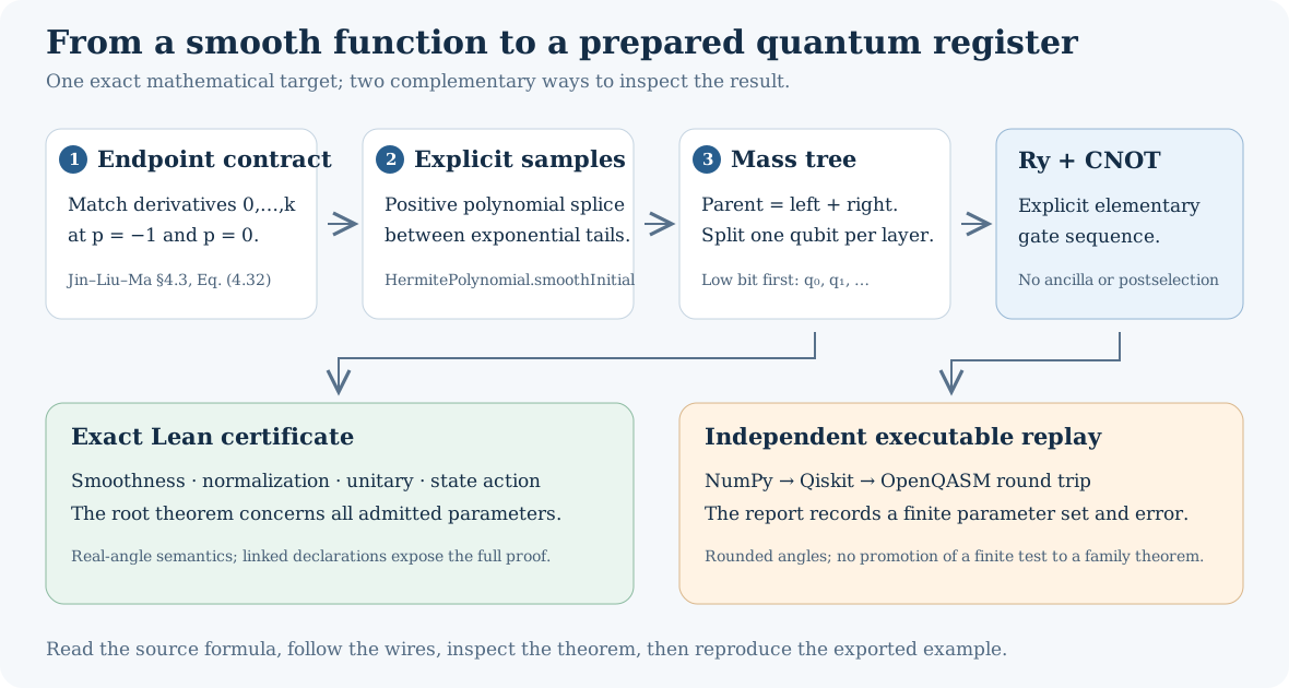
A smooth classical curve becomes the amplitudes of a quantum register.
A generic loader visits exponentially many amplitudes. This particular smooth family has structure: its polynomial piece can be carried by a short vector of Bernstein coefficients, while each exponential tail needs only a scalar update. The new circuit reuses that small memory as it emits the data bits. The original loader remains a transparent reference, not the complexity result.
In Schrödingerisation, this register is prepared independently of the physical-system initial state. Their joint input is \(\lvert g_k\rangle_p\otimes\lvert u_0\rangle\). Subsequent Fourier transforms and evolution are separate algorithm stages.
Read the new circuit first
Follow the data register and the reusable bond register
The data register has \(n_p\) output qubits. The bond register has \(q=\lceil\log_2(2k+6)\rceil\) temporary qubits and must return to \(|0^q\rangle\).
The symbolic tensor train is read most-significant-bit first. Stage \(V_s\) updates the small bond state and emits the next data bit; it does not look up an entry in a length-\(2^{n_p}\) table.
For the tails the update is scalar. For the polynomial branch it carries Bernstein coefficients plus boundary bookkeeping. Before binary padding the total internal dimension is \(D=2k+6\).
Thin LQ/canonicalization makes each stage an isometry; reachable columns are completed to a real unitary and compiled to \(R_y\) and CNOT gates. The final bond sector is clean.
The historical mass-tree/UCRY circuit is retained below as the reference construction. The certified evolution panel shows both routes side by side.
Statement → proof → optional Lean
The mathematical claims, in the order a human would prove them
1 · Source construction
One polynomial satisfies all endpoint derivative conditions
The coefficients are explicit. At the left endpoint all derivatives through order \(k\) equal exp(−1); at the right they alternate between 1 and −1. The polynomial degree is at most 2k+1. The literal piecewise function is globally Cᵏ; a separate gluing theorem closes this analytic claim.
Proof story
- Truncate a formal series\(A_k\) keeps the first \(k+1\) coefficients of \(\exp(t)/(1-t)^{k+1}\). Multiplication restores the exponential coefficients through order \(k\).
- Match each endpointA factor \(t^{k+1}\) kills the first \(k\) derivatives at \(t=0\). Reflect \(t\) to \(1-t\) to obtain the right endpoint.
- Check uniquenessA difference with both zero jets is divisible by \(t^{k+1}(1-t)^{k+1}\), whose degree is too large unless the difference is zero.
- Glue the smooth piecesMatching values and successive derivatives at −1 and 0 gives a globally Cᵏ real function; Lean proves the gluing for arbitrary k.
Show the Lean proof checkpoints
The mathematical explanation above is the reading layer. These compiled declarations are the proof authority.
QuantumBlockEncoding.HermitePolynomial.sourceInterpolant_degreeQuantumBlockEncoding.HermitePolynomial.sourceInterpolant_left_iteratedDerivQuantumBlockEncoding.HermitePolynomial.sourceInterpolant_right_iteratedDerivQuantumBlockEncoding.HermitePolynomial.coefficientPolynomial_evalQuantumBlockEncoding.HermitePolynomial.sourceInterpolant_evalQuantumBlockEncoding.HermitePolynomial.smoothInitial_posQuantumBlockEncoding.HermiteSmoothness.smoothInitial_contDiff
2 · Preparation invariant
The rotations distribute exactly the requested amplitude mass
Every layer resolves one bit of the target state. The squared norm is preserved, and after n layers each leaf amplitude equals its sample divided by the total norm.
Proof story
- Partition by the next bitThe two child index sets are disjoint and together exhaust the parent.
- Apply a two-dimensional rotationCosine and sine give the ratios of child square-root masses to the parent square-root mass.
- Close the rootAt full depth each mass is a single squared sample; normalization and state action follow. Zero-mass subtrees carry zero incoming amplitude.
Show the Lean proof checkpoints
The mathematical explanation above is the reading layer. These compiled declarations are the proof authority.
3 · Polynomial quantum construction
Reuse a small memory instead of listing every amplitude
For every natural \(k\), \(n_p\ge1\) and \(L>0\), an actual Ry/CNOT circuit prepares exactly the same normalized samples. Its small bond memory has \(D\) states before binary padding. Fixed \(k\) therefore gives a linear quantum gate bound in \(n_p\), rather than exponential scaling. No amplitude oracle, success probability or uncharged initial state is assumed. The bound does not yet include the entire classical compiler or finite-bit angle synthesis.
Proof story
- Carry local coefficientsA degree-\(2k+1\) Bernstein vector represents the polynomial piece exactly. A boundary state decides when a dyadic interval enters that piece, and two small tail components handle the exponentials. This gives one consistent chain of width \(2k+6\) for every bit string.
- Normalize without a sample tableSmall local Gram matrices give exactly the full sample norm. Deterministic thin LQ turns the chain into norm-preserving local maps, retaining deficient and zero-rank cases and absorbing the signed first boundary.
- Compile and clean the memoryComplete only the reachable columns to a real unitary, turn each local unitary into selected rotations, and place their Ry/CNOT instructions on the physical wires. The proof covers all output amplitudes, including zero amplitude in every non-clean bond sector.
- Keep the remaining obligations visibleThe raw source now has an actual cached producer with a proved polynomial operation ledger. Stored normalization, LQ, completion and emission still need whole-compiler cost composition. Finite-bit input handling and uniform rounding remain open; finite QASM checks do not fill those gaps.
Show the Lean proof checkpoints
The mathematical explanation above is the reading layer. These compiled declarations are the proof authority.
4 · Classical source construction
Build a short chain, not an exponentially long sample list
The new raw-source producer computes and stores the coefficients, interval boundaries, tail factors and small core matrices. Lean proves that contracting its returned chain gives every original unnormalized sample. The cost bound belongs to this actual producer, not just to the size of a possible representation.
Proof story
- Cache shared workGenerate each reusable coefficient table and tail cache once; carry binary coordinates through the dyadic intervals.
- Keep the original branch testsOnly intervals wholly inside a source piece receive its injection. Both end contractions are retained, including the one-qubit case.
- Read the cost model carefullyThe bound counts declared exact-real operations plus separate exponential and selected integer calls. It does not prove finite-bit runtime or the total cost of compiling the final quantum circuit.
Show the Lean proof checkpoints
The mathematical explanation above is the reading layer. These compiled declarations are the proof authority.
5 · Conditional angle accuracy
A small error per rotation gives a controlled circuit error
Keep every gate in the same position and on the same physical wires. If each changed Ry angle differs by at most delta, the entire constructed circuit differs by at most epsilon in Euclidean operator norm. The bound has no factor proportional to the number of amplitudes.
Proof story
- Control one actual gateThe Ry operator difference is exactly twice the absolute sine of one quarter of the angle difference, hence at most half the angle error.
- Add errors in circuit orderUnitary gates preserve the norm, so the ordered composition accumulates at most half the sum of the per-position angle errors.
- Do not confuse a budget with an implementationA supplied approximate circuit must satisfy that angle accuracy. This theorem does not calculate finite-precision angles, prove a floating-point exporter, or promise exact ancilla cleanup after rounding.
Show the Lean proof checkpoints
The mathematical explanation above is the reading layer. These compiled declarations are the proof authority.
6 · Read the evidence at the correct level
Exact real-angle gates and finite exported circuits answer different questions
The first identity is the symbolic acceptance target. The second is a measured error for a specified exported instance; the acceptance report supplies the parameters, backend versions and tolerances. The measured tolerance here is the maximum componentwise amplitude error, not a whole-vector Euclidean error.
Proof story
- Keep the real-angle semanticsThe generic controlled-rotation compiler preserves the mathematical gate matrix.
- Replay the emitted instructionsNumPy, Qiskit and QASM import all consume the actual elementary-gate list rather than a dense preparation black box.
- Respect the boundaryA small measured error supports that finite export. It neither proves a uniform floating-point bound nor a PDE convergence theorem.
Show the Lean proof checkpoints
The mathematical explanation above is the reading layer. These compiled declarations are the proof authority.
Diagrams and complete source packet
Complete construction and mathematical proof (LaTeX)
Complete construction and mathematical proof (LaTeX)
\documentclass[11pt]{article}
\usepackage{amsmath,amssymb,amsthm,geometry,hyperref}
\geometry{margin=1in}
\newtheorem{theorem}{Theorem}
\newtheorem{lemma}{Lemma}
\newcommand{\ket}[1]{\lvert #1\rangle}
\DeclareMathOperator{\atanTwo}{atan2}
\title{Preparing a Hermite-smoothed quantum initial state}
\author{ASPBE / QuantumComputinglib}
\date{}
\begin{document}
\maketitle

\section{The state, before the circuit}
Fix a nonnegative integer $k$, a register width $n\geq1$, and a truncation
parameter $L>0$. Put $N=2^n$ and $p_j=-\pi L+2\pi Lj/N$ for $0\leq j<N$.
The integer label uses little-endian weights:
$j=\sum_{r=0}^{n-1}2^rq_r$. Thus $q_0$ is the least significant bit,
while the printed ket is $\ket{q_{n-1}\cdots q_0}$.
The required function and quantum state are
\begin{align*}
g_k(p)&=\begin{cases}
 e^p,&p<-1,\\
 P_k(p),&-1\leq p\leq0,\\
 e^{-p},&p>0,
\end{cases}\\
Z_k&=\sum_{j=0}^{N-1}g_k(p_j)^2,
&\ket{g_k}_p&=Z_k^{-1/2}\sum_{j=0}^{N-1}g_k(p_j)\ket j.
\end{align*}
Here $P_k$ has degree at most $2k+1$ and satisfies
\[
P_k^{(a)}(-1)=e^{-1},\qquad P_k^{(a)}(0)=(-1)^a
\quad(0\leq a\leq k).
\]
These are the Hermite conditions in Jin--Liu--Ma,
\emph{Schr\"odingerisation based computationally stable algorithms for
ill-posed problems in partial differential equations},
\href{https://arxiv.org/html/2403.19123v3#S4.SS3}{arXiv:2403.19123v3,
Section 4.3, equations (4.31)--(4.32)}.
The amplitudes are $g_k(p_j)$, not their square roots. The probability of
observing label $j$ is $g_k(p_j)^2/Z_k$.

\section{An explicit polynomial, with no interpolation oracle}
For $0\leq r\leq k$, define
\[
a_{k,r}=\sum_{m=0}^{r}\frac{\binom{k+r-m}{k}}{m!},
\qquad A_k(t)=\sum_{r=0}^{k}a_{k,r}t^r.
\]
With $t=p+1$, set
\[
P_k(p)=e^{-1}(1-t)^{k+1}A_k(t)+t^{k+1}A_k(1-t).
\]
This explicit coefficient formula is the construction used by ASPBE; the
source paper specifies the endpoint conditions.

\begin{lemma}[Endpoint jets and uniqueness]
The displayed polynomial has degree at most $2k+1$ and satisfies all the
Hermite conditions above. No other polynomial of that degree does so.
\end{lemma}
\begin{proof}
The binomial series gives
$(1-t)^{-(k+1)}=\sum_{s\geq0}\binom{k+s}{k}t^s$.
The coefficient of $t^r$ in $e^t(1-t)^{-(k+1)}$ is therefore $a_{k,r}$.
Consequently $(1-t)^{k+1}A_k(t)$ and $e^t$ have identical coefficients
through degree $k$. The other summand contains the factor $t^{k+1}$,
so its first $k$ derivatives vanish at $t=0$. Multiplication by $e^{-1}$
gives the left endpoint values. At $t=1$, exchange $t$ and $1-t$;
each derivative contributes the appropriate factor $(-1)^a$.
Each product has degree at most $2k+1$.
If two interpolants exist, their difference has a zero of multiplicity
at least $k+1$ at both endpoints. It is divisible by
$p^{k+1}(p+1)^{k+1}$, of degree $2k+2$, so the difference is zero.
\end{proof}

\begin{lemma}[Positivity]
The function $g_k$ is positive on the real line; in particular $Z_k>0$.
\end{lemma}
\begin{proof}
All $a_{k,r}$ are positive. For $0<t<1$, both summands in $P_k$ are
positive. At the endpoints their values are $e^{-1}$ and $1$.
The two exterior exponentials are positive as well.
\end{proof}

For $k=1$ the formula reduces to
\[
P_1(p)=(-3+3e^{-1})p^3+(-5+4e^{-1})p^2-p+1.
\]
Its second derivative at zero is $-10+8e^{-1}\ne1$.
Thus the piecewise cubic is $C^1$, not $C^2$. The $C^2$ statement printed
after source equation (6.1) is not adopted here. This case certifies state
preparation; it does not certify the source paper's PDE error estimates.

\section{Construct the rotations from subtree masses}
Write $f_j=g_k(p_j)$. For a depth $d$ and low-bit label $s$, define
\[
m_{d,s}=\sum_{j\bmod 2^d=s}f_j^2,
\quad 0\leq d\leq n,\quad 0\leq s<2^d.
\]
The root mass is $m_{0,0}=Z_k$ and the leaves have $m_{n,j}=f_j^2$.
Partitioning each subtree by its next bit proves
\[
m_{d,s}=m_{d+1,s}+m_{d+1,s+2^d}.
\]
At layer $d$, controlled on $(q_0,\ldots,q_{d-1})$ representing $s$,
apply to $q_d$ the gate
\[
R_y(\theta_{d,s}),\qquad
\theta_{d,s}=2\atanTwo\bigl(\sqrt{m_{d+1,s+2^d}},
                                  \sqrt{m_{d+1,s}}\bigr).
\]
The convention is $R_y(\theta)=
\begin{pmatrix}\cos(\theta/2)&-\sin(\theta/2)\\
\sin(\theta/2)&\cos(\theta/2)\end{pmatrix}$.
For a zero-mass subtree the angle is zero. Its incoming amplitude is already
zero, so this choice does not alter the target.

\begin{theorem}[Deterministic preparation]
The product of these uniformly controlled rotations is unitary and maps
$\ket{0^n}$ to $\ket{g_k}_p$.
\end{theorem}
\begin{proof}
Each fixed control word selects a two-dimensional real rotation. Such a
rotation is orthogonal, hence unitary over the complex numbers. The selected
blocks act on orthogonal control subspaces, and their product is unitary.
After depth $d$ the state is
\[
\sum_{s=0}^{2^d-1}\sqrt{m_{d,s}/Z_k}\,
   \ket{0^{n-d}}\ket{s}.
\]
This holds initially. A rotation splits the amplitude of a parent according
to the square roots of its two child masses, proving the next depth.
At depth $n$, positivity gives $\sqrt{f_j^2}=f_j$, which is the claimed
normalized amplitude. There is no measurement or postselection.
\end{proof}

\section{Global smoothness and exact formal scope}
The endpoint jets also certify that the piecewise function belongs to
$C^k(\mathbb R)$. A generic gluing argument proceeds by induction on the
derivative order: equality of endpoint values gives continuity; equality
of the one-sided derivatives gives differentiability at the junction by
the slope-limit characterization. Applying the induction to the derivative
pieces gives the claim at both junctions.
This is the Lean theorem
\texttt{HermiteSmoothness.smoothInitial\_contDiff}.
The state-preparation root
\texttt{HermiteStatePreparation.hermiteStatePreparation\_complete}
separately certifies normalization, primitive-circuit action, unitarity and
gate counts. Neither root asserts a PDE discretization error, a Sobolev
estimate, or an error bound for machine-rounded angles.

\section{Elementary gates and resource accounting}
A uniformly controlled rotation is compiled recursively using half-sums
and half-differences of its angle table, separated by a CNOT and followed
by a second CNOT. For a control bit $b$, the identity
$X R_y(\beta)X=R_y(-\beta)$ makes the selected angle either
the sum or the difference of the two half-angles.
Induction on the number of controls proves equality of the full matrices.
The reference compiler has $2^d$ rotations and $2(2^d-1)$ CNOTs for $d$
controls. Summing over $d=0,\ldots,n-1$ gives
\[
\#R_y=N-1,\qquad \#\mathrm{CNOT}=2(N-1-n),
\qquad G=3(N-1)-2n.
\]
No auxiliary qubits or state-preparation oracle calls are used. These
counts concern this reference compiler, not an optimality theorem.
Classical coefficient evaluation, sample evaluation, mass reduction and
angle calculation are part of the construction cost. Floating-point
evaluation and angle synthesis are separate from ideal real-angle gates.

\section{Reproduce and inspect the evidence}
The case page links complete Lean modules, the executable generator,
OpenQASM output, a gate diagram, and the numerical acceptance report.
The numerical report records independent NumPy, Qiskit and OpenQASM replay
for finite parameter choices. Those tolerances are not substitutes for
the symbolic Lean state-action theorem. Likewise, the general exact gate
theorem does not assert that machine-rounded rotation angles have zero error.
Every public compilation claim is checked against the repository's current
Lean build before deployment.
\end{document}
Hermite polynomial: complete Lean source
Hermite polynomial: complete Lean source
import Mathlib.Analysis.SpecialFunctions.ExpDeriv
import Mathlib.Analysis.Calculus.Deriv.Polynomial
import Mathlib.Analysis.Calculus.IteratedDeriv.Lemmas
import Mathlib.Algebra.Polynomial.Taylor
import Mathlib.Algebra.Polynomial.FieldDivision
import Mathlib.RingTheory.PowerSeries.Exp
import Mathlib.RingTheory.PowerSeries.WellKnown
import Mathlib.RingTheory.PowerSeries.Trunc
import Mathlib.Tactic

/-!
# Two-point Hermite interpolation for smooth initial data

The source polynomial `sourceInterpolant` is the positive closed form obtained
by truncating `exp(X)/(1-X)^(k+1)`. All endpoint jets and positivity are proved
from its coefficients. An independent extended-Euclid construction is retained
as a reusable two-point interpolation interface. The source contract is the
smooth initial datum in arXiv:2403.19123v3, Section 4.3, equations (4.31)-(4.32).
-/

noncomputable section

open Polynomial

namespace QuantumBlockEncoding.HermitePolynomial

/-- The truncated Taylor polynomial with the prescribed ordinary derivatives. -/
def jetPolynomial (a : ℝ) (k : ℕ) (v : ℕ → ℝ) : ℝ[X] :=
  taylor (-a) (∑ j ∈ Finset.range (k + 1), monomial j (v j / (j.factorial : ℝ)))

/-- Convert Taylor coefficients to ordinary iterated derivatives. -/
theorem eval_iterate_derivative (p : ℝ[X]) (a : ℝ) (j : ℕ) :
    (derivative^[j] p).eval a = (j.factorial : ℝ) * (taylor a p).coeff j := by
  rw [taylor_coeff, ← factorial_smul_hasseDeriv]
  simp [nsmul_eq_mul]

/-- Every requested jet is realized by its local Taylor polynomial. -/
theorem jetPolynomial_jet (a : ℝ) (k j : ℕ) (v : ℕ → ℝ) (hj : j ≤ k) :
    (derivative^[j] (jetPolynomial a k v)).eval a = v j := by
  rw [eval_iterate_derivative]
  simp only [jetPolynomial, taylor_taylor, add_neg_cancel, taylor_zero]
  rw [finset_sum_coeff]
  simp only [coeff_monomial]
  rw [Finset.sum_eq_single j]
  · simp only [ite_true]
    field_simp
  · intro b hb hbj
    simp [hbj]
  · simp [Finset.mem_range, Nat.lt_succ_of_le hj]

/-- A high-multiplicity zero preserves all derivatives below the multiplicity. -/
theorem jet_eq_of_pow_dvd_sub (p q : ℝ[X]) (a : ℝ) (k j : ℕ)
    (hj : j ≤ k) (h : (X - C a) ^ (k + 1) ∣ p - q) :
    (derivative^[j] p).eval a = (derivative^[j] q).eval a := by
  have hd := pow_sub_dvd_iterate_derivative_of_pow_dvd j h
  have hj' : 1 ≤ k + 1 - j := by omega
  have hx' : X - C a ∣ (X - C a) ^ (k + 1 - j) := by
    simpa only [pow_one] using (pow_dvd_pow (X - C a) hj')
  have hx : X - C a ∣ derivative^[j] (p - q) := hx'.trans hd
  obtain ⟨r, hr⟩ := hx
  have he := congrArg (fun f : ℝ[X] => f.eval a) hr
  simpa [iterate_derivative_sub, sub_eq_zero] using he

/-- The inverse constant that normalizes the extended-gcd identity. -/
def bezoutNormalizer (A B : ℝ[X]) : ℝ[X] :=
  C ((EuclideanDomain.gcd A B).coeff 0)⁻¹

theorem bezoutNormalizer_gcd (A B : ℝ[X]) (h : IsCoprime A B) :
    bezoutNormalizer A B * EuclideanDomain.gcd A B = 1 := by
  have hg : IsUnit (EuclideanDomain.gcd A B) :=
    EuclideanDomain.gcd_isUnit_iff.mpr h
  obtain ⟨r, hr, hgr⟩ := Polynomial.isUnit_iff.mp hg
  unfold bezoutNormalizer
  rw [← hgr]
  simp only [coeff_C_zero, ← C_mul, inv_mul_cancel₀ hr.ne_zero, C_1]

/-- An explicit Chinese-remainder interpolant, using extended Euclid. -/
def twoPointInterpolant (A B u v : ℝ[X]) : ℝ[X] :=
  (bezoutNormalizer A B *
    (B * EuclideanDomain.gcdB A B * u + A * EuclideanDomain.gcdA A B * v)) %
    (A * B)

theorem twoPointInterpolant_left (A B u v : ℝ[X]) (h : IsCoprime A B) :
    A ∣ twoPointInterpolant A B u v - u := by
  have he : bezoutNormalizer A B *
      (A * EuclideanDomain.gcdA A B + B * EuclideanDomain.gcdB A B) = 1 := by
    rw [← EuclideanDomain.gcd_eq_gcd_ab]
    exact bezoutNormalizer_gcd A B h
  unfold twoPointInterpolant
  rw [EuclideanDomain.mod_eq_sub_mul_div]
  refine ⟨bezoutNormalizer A B * EuclideanDomain.gcdA A B * (v - u) -
    B * ((bezoutNormalizer A B *
      (B * EuclideanDomain.gcdB A B * u + A * EuclideanDomain.gcdA A B * v)) /
      (A * B)), ?_⟩
  calc
    _ = _ - u * (bezoutNormalizer A B *
        (A * EuclideanDomain.gcdA A B + B * EuclideanDomain.gcdB A B)) := by
      rw [he, mul_one]
    _ = _ := by ring

theorem twoPointInterpolant_right (A B u v : ℝ[X]) (h : IsCoprime A B) :
    B ∣ twoPointInterpolant A B u v - v := by
  have he : bezoutNormalizer A B *
      (A * EuclideanDomain.gcdA A B + B * EuclideanDomain.gcdB A B) = 1 := by
    rw [← EuclideanDomain.gcd_eq_gcd_ab]
    exact bezoutNormalizer_gcd A B h
  unfold twoPointInterpolant
  rw [EuclideanDomain.mod_eq_sub_mul_div]
  refine ⟨bezoutNormalizer A B * EuclideanDomain.gcdB A B * (u - v) -
    A * ((bezoutNormalizer A B *
      (B * EuclideanDomain.gcdB A B * u + A * EuclideanDomain.gcdA A B * v)) /
      (A * B)), ?_⟩
  calc
    _ = _ - v * (bezoutNormalizer A B *
        (A * EuclideanDomain.gcdA A B + B * EuclideanDomain.gcdB A B)) := by
      rw [he, mul_one]
    _ = _ := by ring

/-- The multiplicity polynomial for the endpoint `-1`. -/
def leftModulus (k : ℕ) : ℝ[X] := (X - C (-1)) ^ (k + 1)

/-- The multiplicity polynomial for the endpoint `0`. -/
def rightModulus (k : ℕ) : ℝ[X] := (X - C 0) ^ (k + 1)

theorem endpointModuli_coprime (k : ℕ) : IsCoprime (leftModulus k) (rightModulus k) := by
  apply IsCoprime.pow
  exact isCoprime_X_sub_C_of_isUnit_sub (by norm_num)

/-- The degree-bounded polynomial joining the jets of `exp p` and `exp (-p)`. -/
def interpolant (k : ℕ) : ℝ[X] :=
  twoPointInterpolant (leftModulus k) (rightModulus k)
    (jetPolynomial (-1) k (fun _ => Real.exp (-1)))
    (jetPolynomial 0 k (fun j => (-1 : ℝ) ^ j))

/-- All derivatives through order `k` at `-1` equal `exp (-1)`. -/
theorem interpolant_left_jet (k j : ℕ) (hj : j ≤ k) :
    (derivative^[j] (interpolant k)).eval (-1) = Real.exp (-1) := by
  rw [jet_eq_of_pow_dvd_sub _ (jetPolynomial (-1) k (fun _ => Real.exp (-1)))
    (-1) k j hj]
  · exact jetPolynomial_jet (-1) k j _ hj
  · exact twoPointInterpolant_left _ _ _ _ (endpointModuli_coprime k)

/-- All derivatives through order `k` at `0` equal `(-1)^j`. -/
theorem interpolant_right_jet (k j : ℕ) (hj : j ≤ k) :
    (derivative^[j] (interpolant k)).eval 0 = (-1 : ℝ) ^ j := by
  rw [jet_eq_of_pow_dvd_sub _ (jetPolynomial 0 k (fun j => (-1 : ℝ) ^ j)) 0 k j hj]
  · exact jetPolynomial_jet 0 k j _ hj
  · exact twoPointInterpolant_right _ _ _ _ (endpointModuli_coprime k)

/-- The construction has the minimal Hermite degree bound. -/
theorem interpolant_degree (k : ℕ) : (interpolant k).natDegree ≤ 2 * k + 1 := by
  have hdeg : (leftModulus k * rightModulus k).natDegree = 2 * k + 2 := by
    unfold leftModulus rightModulus
    rw [natDegree_mul (pow_ne_zero _ (X_sub_C_ne_zero _))
      (pow_ne_zero _ (X_sub_C_ne_zero _))]
    simp only [natDegree_pow, natDegree_X_sub_C, mul_one]
    omega
  have h := natDegree_mod_lt
    (bezoutNormalizer (leftModulus k) (rightModulus k) *
      (rightModulus k * EuclideanDomain.gcdB (leftModulus k) (rightModulus k) *
        jetPolynomial (-1) k (fun _ => Real.exp (-1)) +
      leftModulus k * EuclideanDomain.gcdA (leftModulus k) (rightModulus k) *
        jetPolynomial 0 k (fun j => (-1 : ℝ) ^ j)))
    (q := leftModulus k * rightModulus k) (by omega)
  rw [hdeg] at h
  exact Nat.le_of_lt_succ (by simpa [interpolant, twoPointInterpolant, Nat.add_assoc] using h)

/-- The generating series whose first `k+1` coefficients are the source's `a_{k,r}`. -/
def coefficientSeries (k : ℕ) : PowerSeries ℝ :=
  PowerSeries.exp ℝ * (PowerSeries.invOneSubPow ℝ (k + 1)).val

/-- The exact polynomial `A_k`, implemented as a finite Taylor truncation. -/
def coefficientPolynomial (k : ℕ) : ℝ[X] :=
  PowerSeries.trunc (k + 1) (coefficientSeries k)

/-- One endpoint cardinal factor in the symmetric closed-form Hermite formula. -/
def endpointFactor (k : ℕ) : ℝ[X] := (1 - X) ^ (k + 1) * coefficientPolynomial k

/-- The source closed form, in the coordinate `t = p + 1`. -/
def sourceInterpolant (k : ℕ) : ℝ[X] :=
  taylor 1 (C (Real.exp (-1)) * endpointFactor k +
    (endpointFactor k).comp (1 - X))

theorem coefficientSeries_coeff (k r : ℕ) :
    PowerSeries.coeff r (coefficientSeries k) =
      ∑ m ∈ Finset.range (r + 1), (Nat.choose (k + r - m) k : ℝ) /
        (m.factorial : ℝ) := by
  simp only [coefficientSeries, PowerSeries.coeff_mul,
    PowerSeries.invOneSubPow_val_succ_eq_mk_add_choose, PowerSeries.coeff_mk,
    PowerSeries.coeff_exp]
  rw [Finset.Nat.sum_antidiagonal_eq_sum_range_succ_mk]
  apply Finset.sum_congr rfl
  intro m hm
  have hm' : m ≤ r := by simpa using hm
  simp [Nat.add_sub_assoc hm', div_eq_mul_inv, mul_comm]

theorem coefficientSeries_coeff_nonneg (k r : ℕ) :
    0 ≤ PowerSeries.coeff r (coefficientSeries k) := by
  rw [coefficientSeries_coeff]
  exact Finset.sum_nonneg fun _ _ => div_nonneg (Nat.cast_nonneg _) (Nat.cast_nonneg _)

@[simp] theorem coefficientSeries_coeff_zero (k : ℕ) :
    PowerSeries.coeff 0 (coefficientSeries k) = 1 := by
  simp [coefficientSeries_coeff]

theorem endpointFactor_series_trunc (k : ℕ) :
    PowerSeries.trunc (k + 1) (endpointFactor k : PowerSeries ℝ) =
      PowerSeries.trunc (k + 1) (PowerSeries.exp ℝ) := by
  have hi : ((1 - PowerSeries.X : PowerSeries ℝ) ^ (k + 1)) *
      (PowerSeries.invOneSubPow ℝ (k + 1)).val = 1 :=
    (PowerSeries.invOneSubPow ℝ (k + 1)).inv_val
  simp only [endpointFactor, coefficientPolynomial, Polynomial.coe_mul,
    Polynomial.coe_pow, Polynomial.coe_sub, Polynomial.coe_one, Polynomial.coe_X,
    PowerSeries.trunc_mul_trunc, coefficientSeries]
  rw [mul_left_comm, hi, mul_one]

theorem endpointFactor_coeff (k j : ℕ) (hj : j ≤ k) :
    (endpointFactor k).coeff j = 1 / (j.factorial : ℝ) := by
  have he := congrArg (fun p : ℝ[X] => p.coeff j) (endpointFactor_series_trunc k)
  simpa [PowerSeries.coeff_trunc, Nat.lt_succ_of_le hj] using he

theorem endpointFactor_zero_jet (k j : ℕ) (hj : j ≤ k) :
    (derivative^[j] (endpointFactor k)).eval 0 = 1 := by
  rw [eval_iterate_derivative, taylor_zero, endpointFactor_coeff k j hj]
  simp [Nat.factorial_ne_zero]

theorem endpointFactor_one_jet (k j : ℕ) (hj : j ≤ k) :
    (derivative^[j] (endpointFactor k)).eval 1 = 0 := by
  have hf : (X - C (1 : ℝ)) ^ (k + 1) ∣ endpointFactor k - 0 := by
    refine ⟨(-1) ^ (k + 1) * coefficientPolynomial k, ?_⟩
    simp only [endpointFactor, sub_zero, C_1]
    rw [← mul_assoc, ← mul_pow]
    congr 2
    ring
  simpa using jet_eq_of_pow_dvd_sub (endpointFactor k) 0 1 k j hj hf

theorem sourceInterpolant_left_jet (k j : ℕ) (hj : j ≤ k) :
    (derivative^[j] (sourceInterpolant k)).eval (-1) = Real.exp (-1) := by
  rw [eval_iterate_derivative]
  simp only [sourceInterpolant, taylor_taylor, neg_add_cancel, taylor_zero]
  rw [← taylor_zero (C (Real.exp (-1)) * endpointFactor k +
    (endpointFactor k).comp (1 - X)), ← eval_iterate_derivative]
  rw [iterate_map_add, iterate_derivative_C_mul, iterate_derivative_comp_one_sub_X]
  simp [endpointFactor_zero_jet k j hj, endpointFactor_one_jet k j hj]

theorem sourceInterpolant_right_jet (k j : ℕ) (hj : j ≤ k) :
    (derivative^[j] (sourceInterpolant k)).eval 0 = (-1 : ℝ) ^ j := by
  rw [eval_iterate_derivative]
  simp only [sourceInterpolant, taylor_taylor, zero_add]
  rw [← eval_iterate_derivative]
  rw [iterate_map_add, iterate_derivative_C_mul, iterate_derivative_comp_one_sub_X]
  simp [endpointFactor_zero_jet k j hj, endpointFactor_one_jet k j hj]

theorem coefficientPolynomial_pos (k : ℕ) (t : ℝ) (ht : 0 ≤ t) :
    0 < (coefficientPolynomial k).eval t := by
  have hsum : (coefficientPolynomial k).eval t =
      ∑ r ∈ Finset.range (k + 1), PowerSeries.coeff r (coefficientSeries k) * t ^ r :=
    PowerSeries.eval₂_trunc_eq_sum_range t (RingHom.id ℝ) (k + 1) (coefficientSeries k)
  rw [hsum]
  have h := Finset.single_le_sum
    (f := fun r => PowerSeries.coeff r (coefficientSeries k) * t ^ r)
    (fun r _ => mul_nonneg (coefficientSeries_coeff_nonneg k r) (pow_nonneg ht r))
    (show 0 ∈ Finset.range (k + 1) by simp)
  simp only [coefficientSeries_coeff_zero, pow_zero, mul_one] at h
  linarith

theorem sourceInterpolant_pos (k : ℕ) (p : ℝ) (hp : p ∈ Set.Icc (-1) 0) :
    0 < (sourceInterpolant k).eval p := by
  have h0 : 0 ≤ p + 1 := by linarith [hp.1]
  have h1 : 0 ≤ 1 - (p + 1) := by linarith [hp.2]
  have ha := coefficientPolynomial_pos k (p + 1) h0
  have hb := coefficientPolynomial_pos k (1 - (p + 1)) h1
  simp only [sourceInterpolant, taylor_eval, eval_add, eval_mul, eval_C, eval_comp,
    eval_sub, eval_one, eval_X, endpointFactor, eval_pow]
  have he := Real.exp_pos (-1)
  by_cases hz : p + 1 = 0
  · simp only [hz, sub_zero, one_pow, one_mul, zero_pow (Nat.succ_ne_zero k),
      sub_self, zero_mul, add_zero]
    exact mul_pos he (coefficientPolynomial_pos k 0 le_rfl)
  · have ht : 0 < p + 1 := lt_of_le_of_ne h0 (Ne.symm hz)
    have hright : 0 < (1 - (1 - (p + 1))) ^ (k + 1) *
        (coefficientPolynomial k).eval (1 - (p + 1)) := by
      apply mul_pos _ hb
      simpa [add_comm] using pow_pos ht (k + 1)
    exact add_pos_of_nonneg_of_pos
      (mul_nonneg he.le (mul_nonneg (pow_nonneg h1 _) ha.le)) hright

/-- The coefficient polynomial is exactly the finite sum in the closed form. -/
theorem coefficientPolynomial_eval (k : ℕ) (t : ℝ) :
    (coefficientPolynomial k).eval t =
      ∑ r ∈ Finset.range (k + 1),
        (∑ m ∈ Finset.range (r + 1), (Nat.choose (k + r - m) k : ℝ) /
          (m.factorial : ℝ)) * t ^ r := by
  rw [coefficientPolynomial, Polynomial.eval, PowerSeries.eval₂_trunc_eq_sum_range]
  simp only [RingHom.id_apply, coefficientSeries_coeff]

/-- Source formula with the coordinate convention `t = p + 1` made explicit. -/
theorem sourceInterpolant_eval (k : ℕ) (p : ℝ) :
    (sourceInterpolant k).eval p =
      Real.exp (-1) * (1 - (p + 1)) ^ (k + 1) *
        (coefficientPolynomial k).eval (p + 1) +
      (p + 1) ^ (k + 1) * (coefficientPolynomial k).eval (1 - (p + 1)) := by
  simp only [sourceInterpolant, endpointFactor, taylor_eval, eval_add, eval_mul,
    eval_C, eval_pow, eval_sub, eval_one, eval_X, eval_comp]
  congr 1
  · ring
  · congr 2
    ring

theorem coefficientPolynomial_degree (k : ℕ) : (coefficientPolynomial k).natDegree ≤ k :=
  Nat.le_of_lt_succ (PowerSeries.natDegree_trunc_lt (coefficientSeries k) k)

theorem endpointFactor_degree (k : ℕ) : (endpointFactor k).natDegree ≤ 2 * k + 1 := by
  have hs : (1 - X : ℝ[X]).natDegree = 1 := by
    rw [← natDegree_neg]
    simpa using (natDegree_X_sub_C (1 : ℝ))
  have h := natDegree_mul_le (p := (1 - X : ℝ[X]) ^ (k + 1))
    (q := coefficientPolynomial k)
  rw [natDegree_pow, hs, mul_one] at h
  have ha := coefficientPolynomial_degree k
  exact (show (endpointFactor k).natDegree ≤ (k + 1) + (coefficientPolynomial k).natDegree
    from h).trans (by omega)

/-- The source closed form has degree at most `2k+1`. -/
theorem sourceInterpolant_degree (k : ℕ) : (sourceInterpolant k).natDegree ≤ 2 * k + 1 := by
  rw [sourceInterpolant, natDegree_taylor]
  apply natDegree_add_le_of_degree_le
  · exact (natDegree_C_mul_le _ _).trans (endpointFactor_degree k)
  · have hs : (1 - X : ℝ[X]).natDegree = 1 := by
      rw [← natDegree_neg]
      simpa using (natDegree_X_sub_C (1 : ℝ))
    simpa [natDegree_comp, hs] using endpointFactor_degree k

/-- Algebraic and analytic repeated differentiation agree for real polynomials. -/
theorem iteratedDeriv_polynomial (p : ℝ[X]) (j : ℕ) (x : ℝ) :
    iteratedDeriv j (fun y => p.eval y) x = (derivative^[j] p).eval x := by
  induction j generalizing p with
  | zero => rfl
  | succ j ih =>
    rw [iteratedDeriv_succ']
    have he : deriv (fun y => p.eval y) = fun y => p.derivative.eval y := by
      funext y
      exact p.deriv
    rw [he, ih, Function.iterate_succ_apply]

theorem sourceInterpolant_left_iteratedDeriv (k j : ℕ) (hj : j ≤ k) :
    iteratedDeriv j (fun p => (sourceInterpolant k).eval p) (-1) = Real.exp (-1) := by
  rw [iteratedDeriv_polynomial]
  exact sourceInterpolant_left_jet k j hj

theorem sourceInterpolant_right_iteratedDeriv (k j : ℕ) (hj : j ≤ k) :
    iteratedDeriv j (fun p => (sourceInterpolant k).eval p) 0 = (-1 : ℝ) ^ j := by
  rw [iteratedDeriv_polynomial]
  exact sourceInterpolant_right_jet k j hj

/-- The literal piecewise initial datum: left exponential, Hermite bridge, right exponential. -/
def smoothInitial (k : ℕ) (p : ℝ) : ℝ :=
  if p < -1 then Real.exp p else
    if p ≤ 0 then (sourceInterpolant k).eval p else Real.exp (-p)

theorem smoothInitial_left (k : ℕ) (p : ℝ) (hp : p < -1) :
    smoothInitial k p = Real.exp p := by simp [smoothInitial, hp]

theorem smoothInitial_middle (k : ℕ) (p : ℝ) (hp : p ∈ Set.Icc (-1) 0) :
    smoothInitial k p = (sourceInterpolant k).eval p := by
  simp [smoothInitial, not_lt.mpr hp.1, hp.2]

theorem smoothInitial_right (k : ℕ) (p : ℝ) (hp : 0 < p) :
    smoothInitial k p = Real.exp (-p) := by
  simp [smoothInitial, not_lt.mpr (show -1 ≤ p by linarith), not_le.mpr hp]

/-- Strict positivity holds globally and makes every finite sampled norm nonzero. -/
theorem smoothInitial_pos (k : ℕ) (p : ℝ) : 0 < smoothInitial k p := by
  unfold smoothInitial
  split_ifs with hl hr
  · exact Real.exp_pos p
  · exact sourceInterpolant_pos k p ⟨not_lt.mp hl, hr⟩
  · exact Real.exp_pos (-p)

/-- Agreement of a finite jet is equivalent to divisibility by the endpoint multiplicity. -/
theorem pow_dvd_sub_of_jet_eq (p q : ℝ[X]) (a : ℝ) (k : ℕ)
    (h : ∀ j ≤ k, (derivative^[j] p).eval a = (derivative^[j] q).eval a) :
    (X - C a) ^ (k + 1) ∣ p - q := by
  have ht : X ^ (k + 1) ∣ taylor a (p - q) := by
    apply X_pow_dvd_iff.mpr
    intro j hj
    have he : (j.factorial : ℝ) * (taylor a (p - q)).coeff j = 0 := by
      rw [← eval_iterate_derivative]
      simp only [iterate_derivative_sub, eval_sub, h j (by omega), sub_self]
    exact (mul_eq_zero.mp he).resolve_left (by exact_mod_cast Nat.factorial_ne_zero j)
  have hm := map_dvd (taylorAlgHom (-a)) ht
  simpa [taylor_taylor, ← sub_eq_add_neg] using hm

/-- There is only one degree-bounded polynomial with the source endpoint jets. -/
theorem sourceInterpolant_unique (k : ℕ) (p : ℝ[X]) (hp : p.natDegree ≤ 2 * k + 1)
    (hl : ∀ j ≤ k, (derivative^[j] p).eval (-1) = Real.exp (-1))
    (hr : ∀ j ≤ k, (derivative^[j] p).eval 0 = (-1 : ℝ) ^ j) :
    p = sourceInterpolant k := by
  have hleft : leftModulus k ∣ p - sourceInterpolant k :=
    pow_dvd_sub_of_jet_eq p (sourceInterpolant k) (-1) k
      (fun j hj => (hl j hj).trans (sourceInterpolant_left_jet k j hj).symm)
  have hright : rightModulus k ∣ p - sourceInterpolant k :=
    pow_dvd_sub_of_jet_eq p (sourceInterpolant k) 0 k
      (fun j hj => (hr j hj).trans (sourceInterpolant_right_jet k j hj).symm)
  have hdiv := (endpointModuli_coprime k).mul_dvd hleft hright
  by_contra hne
  have hd := natDegree_le_of_dvd hdiv (sub_ne_zero.mpr hne)
  have hm : (leftModulus k * rightModulus k).natDegree = 2 * k + 2 := by
    unfold leftModulus rightModulus
    rw [natDegree_mul (pow_ne_zero _ (X_sub_C_ne_zero _))
      (pow_ne_zero _ (X_sub_C_ne_zero _))]
    simp only [natDegree_pow, natDegree_X_sub_C, mul_one]
    omega
  have hb := (natDegree_sub_le p (sourceInterpolant k)).trans
    (max_le hp (sourceInterpolant_degree k))
  rw [hm] at hd
  omega

/-- The Euclidean-algorithm construction and the positive source formula agree exactly. -/
theorem interpolant_eq_sourceInterpolant (k : ℕ) : interpolant k = sourceInterpolant k :=
  sourceInterpolant_unique k (interpolant k) (interpolant_degree k)
    (interpolant_left_jet k) (interpolant_right_jet k)

end QuantumBlockEncoding.HermitePolynomial
Generic amplitude preparation: complete Lean source
Generic amplitude preparation: complete Lean source
import QuantumBlockEncoding.UniformlyControlledRy
import QuantumBlockEncoding.PrimitiveBasisLE
import QuantumBlockEncoding.StatePreparation

/-!
# Constructive preparation of finite real amplitude tables

Wires are ordered little-endian. The recursive construction prepares the
low-wire marginal norms first, then splits each marginal with a uniformly
controlled rotation on the new highest wire. The angles are exact real
expressions; finite numerical export is a separate evaluation obligation.
-/

namespace QuantumBlockEncoding.RealAmplitudePreparation

open Robin.ComplexLCU
open scoped Kronecker

/-- Adjoin a most-significant bit; existing wire numbers do not change. -/
def lastBasisEquiv (n : Nat) : PrimitiveBasis (n + 1) ≃ PrimitiveBasis n × Fin 2 :=
  (Fin.snocEquiv (fun _ : Fin (n + 1) => Fin 2)).symm.trans (Equiv.prodComm _ _)

@[simp] theorem lastBasisEquiv_apply {n : Nat} (b : PrimitiveBasis (n + 1)) :
    lastBasisEquiv n b = (Fin.init b, b (Fin.last n)) := rfl

@[simp] theorem lastBasisEquiv_symm_apply {n : Nat} (b : PrimitiveBasis n) (v : Fin 2) :
    (lastBasisEquiv n).symm (b, v) = Fin.snoc b v := rfl

theorem basis_eq_iff {n : Nat} (a b : PrimitiveBasis (n + 1)) :
    a = b ↔ Fin.init a = Fin.init b ∧ a (Fin.last n) = b (Fin.last n) := by
  rw [← (lastBasisEquiv n).injective.eq_iff]
  simp

/-- Tensor a circuit matrix with an untouched highest wire. -/
noncomputable def liftLastMatrix {n : Nat}
    (M : _root_.Matrix (PrimitiveBasis n) (PrimitiveBasis n) ℂ) :
    _root_.Matrix (PrimitiveBasis (n + 1)) (PrimitiveBasis (n + 1)) ℂ :=
  _root_.Matrix.reindexAlgEquiv ℂ ℂ (lastBasisEquiv n).symm
    (M ⊗ₖ (1 : _root_.Matrix (Fin 2) (Fin 2) ℂ))

@[simp] theorem liftLastMatrix_apply {n : Nat}
    (M : _root_.Matrix (PrimitiveBasis n) (PrimitiveBasis n) ℂ)
    (a b : PrimitiveBasis (n + 1)) :
    liftLastMatrix M a b =
      if a (Fin.last n) = b (Fin.last n) then M (Fin.init a) (Fin.init b) else 0 := by
  simp [liftLastMatrix, _root_.Matrix.reindexAlgEquiv_apply,
    _root_.Matrix.reindex_apply, _root_.Matrix.submatrix_apply,
    _root_.Matrix.one_apply, mul_ite]

@[simp] theorem liftLastMatrix_one (n : Nat) :
    liftLastMatrix (1 : _root_.Matrix (PrimitiveBasis n) (PrimitiveBasis n) ℂ) = 1 := by
  simp [liftLastMatrix]

theorem liftLastMatrix_mul {n : Nat}
    (M N : _root_.Matrix (PrimitiveBasis n) (PrimitiveBasis n) ℂ) :
    liftLastMatrix (M * N) = liftLastMatrix M * liftLastMatrix N := by
  simp [liftLastMatrix, ← _root_.Matrix.mul_kronecker_mul]

/-- Embed every instruction without changing its original wire number. -/
def liftGate {n : Nat} : PrimitiveGate n → PrimitiveGate (n + 1)
  | .x t => .x t.castSucc
  | .ry t a => .ry t.castSucc a
  | .rz t a => .rz t.castSucc a
  | .cx c t h => .cx c.castSucc t.castSucc (fun e => h (Fin.castSucc_injective _ e))

private theorem split_castSucc_eq {n : Nat} (t : Fin n)
    (a b : PrimitiveBasis (n + 1)) :
    (splitPrimitiveWire t.castSucc a).2 = (splitPrimitiveWire t.castSucc b).2 ↔
      (splitPrimitiveWire t (Fin.init a)).2 = (splitPrimitiveWire t (Fin.init b)).2 ∧
      a (Fin.last n) = b (Fin.last n) := by
  constructor
  · intro h
    constructor
    · funext w
      exact congrFun h ⟨w.1.castSucc, by simpa using w.2⟩
    · exact congrFun h ⟨Fin.last n, Ne.symm (Fin.castSucc_ne_last t)⟩
  · rintro ⟨h, hl⟩
    funext w
    obtain ⟨w, hw⟩ := w
    change a w = b w
    revert hw
    refine Fin.lastCases ?_ (fun i => ?_) w
    · intro _; exact hl
    · intro hi
      exact congrFun h ⟨i, by simpa using hi⟩

theorem lift_oneQubit {n : Nat} (t : Fin n)
    (M : _root_.Matrix (Fin 2) (Fin 2) ℂ) :
    liftPrimitiveOneQubit t.castSucc M = liftLastMatrix (liftPrimitiveOneQubit t M) := by
  ext a b
  simp only [liftPrimitiveOneQubit_apply, liftLastMatrix_apply, split_castSucc_eq]
  by_cases hc : (splitPrimitiveWire t (Fin.init a)).2 =
      (splitPrimitiveWire t (Fin.init b)).2 <;>
    by_cases hl : a (Fin.last n) = b (Fin.last n) <;>
    simp [hc, hl, Fin.init]

private theorem xBasis_lift {n : Nat} (t : Fin n) (b : PrimitiveBasis (n + 1)) :
    Fin.init (xBasisAction t.castSucc b) = xBasisAction t (Fin.init b) := by
  funext i
  simp [xBasisAction, Fin.init, Function.update_apply]

private theorem cxBasis_lift {n : Nat} (c t : Fin n) (b : PrimitiveBasis (n + 1)) :
    Fin.init (cxBasisAction c.castSucc t.castSucc b) =
      cxBasisAction c t (Fin.init b) := by
  by_cases h : b c.castSucc = 0 <;>
    simp [cxBasisAction, h, Fin.init, xBasis_lift]

theorem eval_liftGate {n : Nat} (g : PrimitiveGate n) :
    evalPrimitiveGate (liftGate g) = liftLastMatrix (evalPrimitiveGate g) := by
  cases g with
  | ry t a => exact lift_oneQubit t _
  | rz t a => exact lift_oneQubit t _
  | x t =>
    ext a b
    simp only [liftGate, evalPrimitiveGate, equivPermutationMatrix, liftLastMatrix_apply]
    change (if a = xBasisAction t.castSucc b then 1 else 0) =
      if a (Fin.last n) = b (Fin.last n) then
        if Fin.init a = xBasisAction t (Fin.init b) then 1 else 0 else 0
    have hl : xBasisAction t.castSucc b (Fin.last n) = b (Fin.last n) := by
      simp [xBasisAction, Ne.symm (Fin.castSucc_ne_last t)]
    simp only [basis_eq_iff, xBasis_lift, hl]
    by_cases h : a (Fin.last n) = b (Fin.last n) <;> simp [h]
  | cx c t h =>
    ext a b
    simp only [liftGate, evalPrimitiveGate, equivPermutationMatrix, liftLastMatrix_apply]
    change (if a = cxBasisAction c.castSucc t.castSucc b then 1 else 0) =
      if a (Fin.last n) = b (Fin.last n) then
        if Fin.init a = cxBasisAction c t (Fin.init b) then 1 else 0 else 0
    have hl : cxBasisAction c.castSucc t.castSucc b (Fin.last n) = b (Fin.last n) := by
      by_cases hc : b c.castSucc = 0 <;>
        simp [cxBasisAction, hc, xBasisAction, Ne.symm (Fin.castSucc_ne_last t)]
    simp only [basis_eq_iff, cxBasis_lift, hl]
    by_cases h : a (Fin.last n) = b (Fin.last n) <;> simp [h]

theorem eval_liftCircuit {n : Nat} (c : PrimitiveCircuit n) :
    evalPrimitiveCircuit (c.map liftGate) = liftLastMatrix (evalPrimitiveCircuit c) := by
  induction c with
  | nil => simp [evalPrimitiveCircuit]
  | cons g c ih =>
    simp only [List.map_cons, evalPrimitiveCircuit, ih, eval_liftGate, liftLastMatrix_mul]

/-- Euclidean mass at one binary split. -/
noncomputable def pairNorm (a b : ℝ) : ℝ := Real.sqrt (a ^ 2 + b ^ 2)

theorem pairNorm_nonneg (a b : ℝ) : 0 ≤ pairNorm a b := Real.sqrt_nonneg _

theorem pairNorm_sq (a b : ℝ) : pairNorm a b ^ 2 = a ^ 2 + b ^ 2 := by
  exact Real.sq_sqrt (add_nonneg (sq_nonneg a) (sq_nonneg b))

/-- Twice the signed polar angle, with the zero subtree assigned angle zero.
The arccos formula avoids an unverified numerical `atan2` primitive. -/
noncomputable def splitAngle (a b : ℝ) : ExactAngle :=
  if pairNorm a b = 0 then .rational 0 else
    .real (2 * if b < 0 then -Real.arccos (a / pairNorm a b)
      else Real.arccos (a / pairNorm a b))

theorem splitAngle_firstColumn (a b : ℝ) (v : Fin 2) :
    standardRyMatrix (splitAngle a b).eval v 0 * (pairNorm a b : ℂ) =
      if v = 0 then (a : ℂ) else (b : ℂ) := by
  have hr := pairNorm_nonneg a b
  have hr2 := pairNorm_sq a b
  by_cases hz : pairNorm a b = 0
  · have ha : a = 0 := by nlinarith [sq_nonneg b]
    have hb : b = 0 := by nlinarith [sq_nonneg a]
    rw [hz, Complex.ofReal_zero, mul_zero]
    simp [ha, hb]
  · have hp : 0 < pairNorm a b := lt_of_le_of_ne hr (Ne.symm hz)
    have ha : -pairNorm a b ≤ a ∧ a ≤ pairNorm a b := by
      constructor <;> nlinarith [sq_nonneg b]
    have lower : -1 ≤ a / pairNorm a b := (le_div_iff₀ hp).2 (by linarith)
    have upper : a / pairNorm a b ≤ 1 := (div_le_iff₀ hp).2 (by linarith)
    have hc : Real.cos (Real.arccos (a / pairNorm a b)) * pairNorm a b = a := by
      rw [Real.cos_arccos lower upper, div_mul_cancel₀ _ hz]
    have hs : 0 ≤ Real.sin (Real.arccos (a / pairNorm a b)) * pairNorm a b :=
      mul_nonneg (Real.sin_nonneg_of_nonneg_of_le_pi
        (Real.arccos_nonneg _) (Real.arccos_le_pi _)) hr
    have hs2 : (Real.sin (Real.arccos (a / pairNorm a b)) * pairNorm a b) ^ 2 = b ^ 2 := by
      have h := congrArg (fun x : ℝ => x * pairNorm a b ^ 2)
        (Real.sin_sq_add_cos_sq (Real.arccos (a / pairNorm a b)))
      nlinarith [sq_nonneg (Real.sin (Real.arccos (a / pairNorm a b)) * pairNorm a b)]
    have hangle : (2 * (if b < 0 then -Real.arccos (a / pairNorm a b)
        else Real.arccos (a / pairNorm a b))) / 2 =
        if b < 0 then -Real.arccos (a / pairNorm a b) else Real.arccos (a / pairNorm a b) := by
      ring
    simp only [splitAngle, if_neg hz, ExactAngle.eval, standardRyMatrix]
    rw [hangle]
    fin_cases v <;> by_cases hb : b < 0
    · simpa only [if_pos hb, realRotation, realOrthogonalRotation, Fin.val_zero,
        Real.cos_neg, if_pos rfl, Complex.ofReal_mul] using congrArg Complex.ofReal hc
    · simpa only [if_neg hb, realRotation, realOrthogonalRotation, Fin.val_zero,
        if_pos rfl, Complex.ofReal_mul] using congrArg Complex.ofReal hc
    · have he : -(Real.sin (Real.arccos (a / pairNorm a b)) * pairNorm a b) = b := by
        nlinarith
      simpa only [if_pos hb, realRotation, realOrthogonalRotation, Fin.val_zero,
        Fin.val_one, Real.sin_neg, Complex.ofReal_neg, Complex.ofReal_mul,
        neg_mul, show (1 : Fin 2) ≠ 0 from by decide, if_false] using congrArg Complex.ofReal he
    · have he : Real.sin (Real.arccos (a / pairNorm a b)) * pairNorm a b = b := by
        nlinarith
      simpa only [if_neg hb, realRotation, realOrthogonalRotation, Fin.val_zero,
        Fin.val_one, Complex.ofReal_mul,
        show (1 : Fin 2) ≠ 0 from by decide, if_false] using congrArg Complex.ofReal he

/-- Marginal amplitudes on all but the highest wire. -/
noncomputable def marginal {n : Nat} (f : PrimitiveBasis (n + 1) → ℝ) :
    PrimitiveBasis n → ℝ := fun b => pairNorm (f (Fin.snoc b 0)) (f (Fin.snoc b 1))

theorem marginal_nonneg {n : Nat} (f : PrimitiveBasis (n + 1) → ℝ) (b : PrimitiveBasis n) :
    0 ≤ marginal f b := pairNorm_nonneg _ _

/-- True squared Euclidean norm of the complete amplitude table. -/
noncomputable def normSq {n : Nat} (f : PrimitiveBasis n → ℝ) : ℝ := ∑ b, f b ^ 2

theorem normSq_nonneg {n : Nat} (f : PrimitiveBasis n → ℝ) : 0 ≤ normSq f :=
  Finset.sum_nonneg (fun _ _ => sq_nonneg _)

theorem normSq_marginal {n : Nat} (f : PrimitiveBasis (n + 1) → ℝ) :
    normSq (marginal f) = normSq f := by
  unfold normSq
  simp only [marginal, pairNorm_sq]
  rw [← (lastBasisEquiv n).symm.sum_comp]
  simp [Fintype.sum_prod_type, Fin.sum_univ_two]

/-- Chronological low-bit-first binary tree, compiled entirely to RY and CX. -/
noncomputable def prepareCircuit : (n : Nat) → (PrimitiveBasis n → ℝ) → PrimitiveCircuit n
  | 0, _ => []
  | n + 1, f =>
    (prepareCircuit n (marginal f)).map liftGate ++
      compileUniformlyControlledRy n Fin.castSucc (Fin.last n) Fin.castSucc_ne_last
        (fun b => splitAngle (f (Fin.snoc b 0)) (f (Fin.snoc b 1)))

theorem prepareCircuit_unitary {n : Nat} (f : PrimitiveBasis n → ℝ) :
    evalPrimitiveCircuit (prepareCircuit n f) ∈
      _root_.Matrix.unitaryGroup (PrimitiveBasis n) ℂ :=
  evalPrimitiveCircuit_unitary _

private theorem last_context_eq {n : Nat} (a b : PrimitiveBasis (n + 1)) :
    (splitPrimitiveWire (Fin.last n) a).2 = (splitPrimitiveWire (Fin.last n) b).2 ↔
      Fin.init a = Fin.init b := by
  constructor
  · intro h
    funext i
    exact congrFun h ⟨i.castSucc, Fin.castSucc_ne_last i⟩
  · intro h
    funext w
    obtain ⟨w, hw⟩ := w
    change a w = b w
    revert hw
    refine Fin.lastCases ?_ (fun i => ?_) w
    · intro h; exact (h rfl).elim
    · intro _; exact congrFun h i

theorem controlledLast_apply {n : Nat} (angles : PrimitiveBasis n → ExactAngle)
    (a b : PrimitiveBasis (n + 1)) :
    controlledRyBlockMatrix Fin.castSucc (Fin.last n) Fin.castSucc_ne_last angles a b =
      if Fin.init a = Fin.init b then
        standardRyMatrix (angles (Fin.init a)).eval (a (Fin.last n)) (b (Fin.last n))
      else 0 := by
  simp only [controlledRyBlockMatrix_apply, last_context_eq]
  rfl

theorem controlledLast_mul_lift {n : Nat} (angles : PrimitiveBasis n → ExactAngle)
    (M : _root_.Matrix (PrimitiveBasis n) (PrimitiveBasis n) ℂ)
    (a : PrimitiveBasis (n + 1)) :
    (controlledRyBlockMatrix Fin.castSucc (Fin.last n) Fin.castSucc_ne_last angles *
        liftLastMatrix M) a (fun _ => 0) =
      standardRyMatrix (angles (Fin.init a)).eval (a (Fin.last n)) 0 *
        M (Fin.init a) (fun _ => 0) := by
  rw [_root_.Matrix.mul_apply, ← (lastBasisEquiv n).symm.sum_comp]
  simp only [controlledLast_apply, liftLastMatrix_apply]
  simp [Fintype.sum_prod_type]
  exact Or.inl rfl

/-- The compiled first column is the normalized input table. This version
also covers the zero-qubit register, whose sole amplitude must be nonnegative. -/
theorem prepareCircuit_firstColumn {n : Nat} (f : PrimitiveBasis n → ℝ)
    (nonneg : ∀ b, 0 ≤ f b) (positive : 0 < normSq f) (b : PrimitiveBasis n) :
    evalPrimitiveCircuit (prepareCircuit n f) b (fun _ => 0) =
      ((f b / Real.sqrt (normSq f) : ℝ) : ℂ) := by
  induction n with
  | zero =>
    have heq : b = (fun _ => 0) := Subsingleton.elim _ _
    have hnorm : normSq f = f b ^ 2 := by
      calc
        normSq f = ∑ _x : PrimitiveBasis 0, f b ^ 2 :=
          Finset.sum_congr rfl (fun x _ => congrArg (fun x => f x ^ 2) (Subsingleton.elim x b))
        _ = f b ^ 2 := by simp
    have hf : 0 < f b := by have := nonneg b; rw [hnorm] at positive; nlinarith
    rw [hnorm, Real.sqrt_sq (le_of_lt hf), div_self (ne_of_gt hf)]
    simp [prepareCircuit, evalPrimitiveCircuit, heq]
  | succ n ih =>
    simp only [prepareCircuit, evalPrimitiveCircuit_append, eval_liftCircuit,
      compileUniformlyControlledRy_eval_controlledRyBlockMatrix]
    rw [controlledLast_mul_lift]
    rw [ih (marginal f) (marginal_nonneg f) (by simpa [normSq_marginal] using positive)]
    rw [normSq_marginal]
    push_cast
    rw [← mul_div_assoc]
    change
      (standardRyMatrix
        (splitAngle (f (Fin.snoc (Fin.init b) 0)) (f (Fin.snoc (Fin.init b) 1))).eval
          (b (Fin.last n)) 0 *
        (pairNorm (f (Fin.snoc (Fin.init b) 0)) (f (Fin.snoc (Fin.init b) 1)) : ℂ)) /
          (Real.sqrt (normSq f) : ℂ) = _
    rw [splitAngle_firstColumn]
    congr 1
    have hs : Fin.snoc (Fin.init b) (b (Fin.last n)) = b := Fin.snoc_init_self b
    generalize hv : b (Fin.last n) = v at *
    fin_cases v <;> simp_all

/-- Normalization is the actual sum of squared amplitudes, not a certificate flag. -/
theorem normalized_sum_sq {n : Nat} (f : PrimitiveBasis n → ℝ)
    (positive : 0 < normSq f) :
    (∑ b, (f b / Real.sqrt (normSq f)) ^ 2) = 1 := by
  simp_rw [div_pow]
  rw [← Finset.sum_div]
  change normSq f / Real.sqrt (normSq f) ^ 2 = 1
  rw [Real.sq_sqrt (normSq_nonneg f), div_self (ne_of_gt positive)]

theorem normSq_pos_of_positive {n : Nat} (f : PrimitiveBasis n → ℝ)
    (positive : ∀ b, 0 < f b) : 0 < normSq f := by
  apply Finset.sum_pos
  · intro b _; exact sq_pos_of_pos (positive b)
  · exact Finset.univ_nonempty

theorem liftCircuit_ryCount {n : Nat} (c : PrimitiveCircuit n) :
    PrimitiveCircuit.ryCount (c.map liftGate) = c.ryCount := by
  induction c with
  | nil => rfl
  | cons g c ih =>
    cases g <;> simp_all [PrimitiveCircuit.ryCount, liftGate]

theorem liftCircuit_cxCount {n : Nat} (c : PrimitiveCircuit n) :
    PrimitiveCircuit.cxCount (c.map liftGate) = c.cxCount := by
  induction c with
  | nil => rfl
  | cons g c ih =>
    cases g <;> simp_all [PrimitiveCircuit.cxCount, liftGate]

/-- The unoptimized reference tree uses exactly one RY per internal tree node. -/
theorem prepareCircuit_ryCount {n : Nat} (f : PrimitiveBasis n → ℝ) :
    (prepareCircuit n f).ryCount = 2 ^ n - 1 := by
  induction n with
  | zero => rfl
  | succ n ih =>
    simp only [prepareCircuit, PrimitiveCircuit.ryCount_append, liftCircuit_ryCount,
      compileUniformlyControlledRy_ryCount, ih, pow_succ]
    have hp : 0 < 2 ^ n := pow_pos (by decide) _
    omega

/-- CX count for the recursive reference multiplexor, without Gray-code optimization. -/
theorem prepareCircuit_cxCount {n : Nat} (f : PrimitiveBasis n → ℝ) :
    (prepareCircuit n f).cxCount = 2 * (2 ^ n - 1 - n) := by
  induction n with
  | zero => rfl
  | succ n ih =>
    simp only [prepareCircuit, PrimitiveCircuit.cxCount_append, liftCircuit_cxCount,
      compileUniformlyControlledRy_cxCount, ih, pow_succ]
    have hp : n < 2 ^ n := Nat.lt_two_pow_self
    omega

theorem prepareCircuit_oracleCalls {n : Nat} (f : PrimitiveBasis n → ℝ) :
    (prepareCircuit n f).resource.oracleCalls = 0 :=
  PrimitiveCircuit.resource_oracleCalls_eq_zero _

@[simp] theorem primitiveBasisLE_zero (n : Nat) :
    primitiveBasisLEEquiv n (fun _ => 0) = zeroBasisIndex n := by
  apply Fin.ext
  induction n with
  | zero => rfl
  | succ n ih =>
    change 0 + 2 * (primitiveBasisLEEquiv n (fun _ => 0)).val = 0
    simpa using congrArg (fun x : Nat => 2 * x) ih

@[simp] theorem primitiveBasisLE_zero_symm (n : Nat) :
    (primitiveBasisLEEquiv n).symm (zeroBasisIndex n) = (fun _ => 0) := by
  apply (primitiveBasisLEEquiv n).injective
  simp

/-- The same circuit matrix on flat little-endian integer indices. -/
noncomputable def prepareMatrixLE {n : Nat} (f : Fin (gridSize n) → ℝ) :
    _root_.Matrix (Fin (gridSize n)) (Fin (gridSize n)) ℂ :=
  _root_.Matrix.reindexAlgEquiv ℂ ℂ (primitiveBasisLEEquiv n)
    (evalPrimitiveCircuit (prepareCircuit n (fun b => f (primitiveBasisLEEquiv n b))))

theorem prepareMatrixLE_unitary {n : Nat} (f : Fin (gridSize n) → ℝ) :
    prepareMatrixLE f ∈ _root_.Matrix.unitaryGroup (Fin (gridSize n)) ℂ :=
  reindex_unitary _ _ (prepareCircuit_unitary _)

theorem normSq_reindex {n : Nat} (f : Fin (gridSize n) → ℝ) :
    normSq (fun b => f (primitiveBasisLEEquiv n b)) = ∑ j, f j ^ 2 := by
  exact (primitiveBasisLEEquiv n).sum_comp (fun j => f j ^ 2)

theorem prepareMatrixLE_firstColumn {n : Nat} (f : Fin (gridSize n) → ℝ)
    (positive : ∀ j, 0 < f j) (j : Fin (gridSize n)) :
    prepareMatrixLE f j (zeroBasisIndex n) =
      ((f j / Real.sqrt (∑ i, f i ^ 2) : ℝ) : ℂ) := by
  unfold prepareMatrixLE
  simp only [_root_.Matrix.reindexAlgEquiv_apply, _root_.Matrix.reindex_apply,
    _root_.Matrix.submatrix_apply, primitiveBasisLE_zero_symm]
  rw [prepareCircuit_firstColumn _ (fun b => le_of_lt (positive _))
    (normSq_pos_of_positive _ (fun b => positive _)), normSq_reindex]
  simp

theorem normalized_sum_sq_LE {n : Nat} (f : Fin (gridSize n) → ℝ)
    (positive : ∀ j, 0 < f j) :
    (∑ j, (f j / Real.sqrt (∑ i, f i ^ 2)) ^ 2) = 1 := by
  have h := normalized_sum_sq (fun b => f (primitiveBasisLEEquiv n b))
    (normSq_pos_of_positive _ (fun b => positive _))
  rw [normSq_reindex] at h
  calc
    _ = ∑ b, (f (primitiveBasisLEEquiv n b) / Real.sqrt (∑ i, f i ^ 2)) ^ 2 :=
      ((primitiveBasisLEEquiv n).sum_comp _).symm
    _ = 1 := h

end QuantumBlockEncoding.RealAmplitudePreparation
Global Cᵏ smoothness: complete Lean source
Global Cᵏ smoothness: complete Lean source
import QuantumBlockEncoding.HermitePolynomial
import Mathlib.Analysis.Calculus.ContDiff.Polynomial
import Mathlib.Analysis.Calculus.Deriv.Slope
import Mathlib.Topology.Piecewise

/-!
# Global regularity of the Hermite initial datum

Matching derivatives are used to prove a reusable finite-order gluing theorem.
Applying that theorem at both source junctions proves global `C^k` regularity
of the actual exponential/Hermite/exponential function.
-/

noncomputable section

open Filter Set Topology Polynomial
open QuantumBlockEncoding.HermitePolynomial

namespace QuantumBlockEncoding.HermiteSmoothness

/-- Join two real functions at a threshold, taking the right value at the threshold. -/
def splice (c : ℝ) (f g : ℝ → ℝ) (x : ℝ) : ℝ := if x < c then f x else g x

/-- Any selector preserves a common derivative when both branch values agree. -/
theorem hasDerivAt_ite_of_eq (pred : ℝ → Prop) [DecidablePred pred]
    {f g : ℝ → ℝ} {d x : ℝ} (hf : HasDerivAt f d x) (hg : HasDerivAt g d x)
    (hv : f x = g x) :
    HasDerivAt (fun y => if pred y then f y else g y) d x := by
  apply hasDerivAt_iff_tendsto_slope.mpr
  have he : slope (fun y => if pred y then f y else g y) x =
      fun y => if pred y then slope f x y else slope g x y := by
    funext y
    by_cases hx : pred x <;> by_cases hy : pred y <;>
      simp [slope_def_field, hx, hy, hv]
  rw [he]
  exact hf.tendsto_slope.if' hg.tendsto_slope

theorem hasDerivAt_splice (c : ℝ) (f g : ℝ → ℝ)
    (hf : Differentiable ℝ f) (hg : Differentiable ℝ g)
    (hv : f c = g c) (hd : deriv f c = deriv g c) (x : ℝ) :
    HasDerivAt (splice c f g) (splice c (deriv f) (deriv g) x) x := by
  rcases lt_trichotomy x c with hx | hxc | hx
  · rw [splice, if_pos hx]
    apply (hf x).hasDerivAt.congr_of_eventuallyEq
    filter_upwards [eventually_lt_nhds hx] with y hy
    simp [splice, hy]
  · subst x
    simp only [splice, lt_self_iff_false, if_false]
    exact hasDerivAt_ite_of_eq (fun y => y < c)
      (hd ▸ (hf c).hasDerivAt) (hg c).hasDerivAt hv
  · rw [splice, if_neg (not_lt.mpr hx.le)]
    apply (hg x).hasDerivAt.congr_of_eventuallyEq
    filter_upwards [eventually_gt_nhds hx] with y hy
    simp [splice, not_lt.mpr hy.le]

theorem deriv_splice (c : ℝ) (f g : ℝ → ℝ)
    (hf : Differentiable ℝ f) (hg : Differentiable ℝ g)
    (hv : f c = g c) (hd : deriv f c = deriv g c) :
    deriv (splice c f g) = splice c (deriv f) (deriv g) := by
  funext x
  exact (hasDerivAt_splice c f g hf hg hv hd x).deriv

/-- Two `C^k` real functions glue to a `C^k` function if their jets agree at the cut. -/
theorem contDiff_splice (k : ℕ) (c : ℝ) (f g : ℝ → ℝ)
    (hf : ContDiff ℝ k f) (hg : ContDiff ℝ k g)
    (hjet : ∀ j ≤ k, iteratedDeriv j f c = iteratedDeriv j g c) :
    ContDiff ℝ k (splice c f g) := by
  induction k generalizing f g with
  | zero =>
    rw [Nat.cast_zero, contDiff_zero]
    apply Continuous.if ?_ hf.continuous hg.continuous
    intro x hx
    have hxc : x = c := by
      change x ∈ frontier (Iio c) at hx
      simpa only [frontier_Iio, mem_singleton_iff] using hx
    subst x
    simpa using hjet 0 le_rfl
  | succ k ih =>
    rw [Nat.cast_add, Nat.cast_one] at hf hg ⊢
    obtain ⟨hfd, _, hfder⟩ := contDiff_succ_iff_deriv.mp hf
    obtain ⟨hgd, _, hgder⟩ := contDiff_succ_iff_deriv.mp hg
    have hv : f c = g c := by simpa using hjet 0 (Nat.zero_le _)
    have hd : deriv f c = deriv g c := by simpa using hjet 1 (by omega)
    apply contDiff_succ_iff_deriv.mpr
    refine ⟨fun x => (hasDerivAt_splice c f g hfd hgd hv hd x).differentiableAt,
      by simp, ?_⟩
    rw [deriv_splice c f g hfd hgd hv hd]
    apply ih (deriv f) (deriv g) hfder hgder
    intro j hj
    simpa only [iteratedDeriv_succ'] using hjet (j + 1) (by omega)

theorem iteratedDeriv_exp (j : ℕ) (x : ℝ) : iteratedDeriv j Real.exp x = Real.exp x := by
  simpa using congrFun (iteratedDeriv_exp_const_mul j (1 : ℝ)) x

theorem iteratedDeriv_exp_neg (j : ℕ) (x : ℝ) :
    iteratedDeriv j (fun y : ℝ => Real.exp (-y)) x = (-1 : ℝ) ^ j * Real.exp (-x) := by
  simpa using congrFun (iteratedDeriv_exp_const_mul j (-1 : ℝ)) x

/-- First join: the source polynomial and right exponential meet smoothly at zero. -/
theorem contDiff_right_splice (k : ℕ) :
    ContDiff ℝ k
      (splice 0 (fun p => (sourceInterpolant k).eval p) (fun p => Real.exp (-p))) := by
  apply contDiff_splice k 0
  · simpa using (sourceInterpolant k).contDiff_aeval (k : WithTop ℕ∞)
  · exact Real.contDiff_exp.comp contDiff_id.neg
  · intro j hj
    rw [sourceInterpolant_right_iteratedDeriv k j hj, iteratedDeriv_exp_neg]
    simp

/-- The right splice coincides with the polynomial on a neighborhood of the left junction. -/
theorem right_splice_eventuallyEq (k : ℕ) :
    splice 0 (fun p => (sourceInterpolant k).eval p) (fun p => Real.exp (-p))
      =ᶠ[𝓝 (-1)] (fun p => (sourceInterpolant k).eval p) := by
  filter_upwards [eventually_lt_nhds (show (-1 : ℝ) < 0 by norm_num)] with p hp
  simp [splice, hp]

/-- Two applications of the reusable gluing theorem close both source junctions. -/
theorem contDiff_double_splice (k : ℕ) :
    ContDiff ℝ k
      (splice (-1) Real.exp
        (splice 0 (fun p => (sourceInterpolant k).eval p) (fun p => Real.exp (-p)))) := by
  apply contDiff_splice k (-1) Real.exp _ Real.contDiff_exp (contDiff_right_splice k)
  intro j hj
  rw [iteratedDeriv_exp, (right_splice_eventuallyEq k).iteratedDeriv_eq j]
  exact (sourceInterpolant_left_iteratedDeriv k j hj).symm

/-- The original `≤ 0` middle-branch convention equals the smooth double splice exactly. -/
theorem smoothInitial_eq_double_splice (k : ℕ) :
    smoothInitial k = splice (-1) Real.exp
      (splice 0 (fun p => (sourceInterpolant k).eval p) (fun p => Real.exp (-p))) := by
  funext p
  by_cases hl : p < -1
  · simp [smoothInitial, splice, hl]
  · by_cases hr : p < 0
    · simp [smoothInitial, splice, hl, hr, hr.le]
    · by_cases hz : p = 0
      · subst p
        have hp0 : (sourceInterpolant k).eval 0 = 1 := by
          simpa using sourceInterpolant_right_jet k 0 (Nat.zero_le k)
        simp [smoothInitial, splice, hp0]
      · have hp : 0 < p := lt_of_le_of_ne (not_lt.mp hr) (Ne.symm hz)
        simp [smoothInitial, splice, hl, hr, not_le.mpr hp]

/-- The literal source initial datum is globally `C^k`, for every natural order `k`. -/
theorem smoothInitial_contDiff (k : ℕ) : ContDiff ℝ k (smoothInitial k) := by
  rw [smoothInitial_eq_double_splice]
  exact contDiff_double_splice k

end QuantumBlockEncoding.HermiteSmoothness
Hermite target and root certificate: complete Lean source
Hermite target and root certificate: complete Lean source
import QuantumBlockEncoding.HermitePolynomial
import QuantumBlockEncoding.RealAmplitudePreparation

/-!
# Exact Hermite smooth-initial-data preparation

The target is the literal exponential / Hermite-polynomial / exponential
splice, sampled at `p_j = -πL + 2πLj / 2^n`. The unitary below is the denotation
of an explicit RY/CX circuit. Its first column, normalization, and reference
gate counts hold for every smoothing order and register width.

Exact real angles belong to the symbolic certificate. Numerical evaluation
and rounded QASM angles remain separate executable-export evidence.
-/

namespace QuantumBlockEncoding.HermiteStatePreparation

open HermitePolynomial RealAmplitudePreparation ConcreteSemantics

noncomputable section

/-- Left-inclusive, right-exclusive grid on `[-πL,πL)` when `L>0`. -/
def gridPoint (n : ℕ) (L : ℝ) (j : Fin (gridSize n)) : ℝ :=
  -Real.pi * L + (j.val : ℝ) * (2 * Real.pi * L / (gridSize n : ℝ))

/-- The physical sample, without changing the polynomial on the splice interval. -/
def sampledAmplitude (k n : ℕ) (L : ℝ) (j : Fin (gridSize n)) : ℝ :=
  smoothInitial k (gridPoint n L j)

theorem sampledAmplitude_pos (k n : ℕ) (L : ℝ) (j : Fin (gridSize n)) :
    0 < sampledAmplitude k n L j := smoothInitial_pos _ _

/-- The true Euclidean normalizer of the complete finite sample table. -/
def sampleNorm (k n : ℕ) (L : ℝ) : ℝ :=
  Real.sqrt (∑ j, sampledAmplitude k n L j ^ 2)

theorem sampleNorm_pos (k n : ℕ) (L : ℝ) : 0 < sampleNorm k n L := by
  apply Real.sqrt_pos.mpr
  have h := normSq_pos_of_positive
    (fun b => sampledAmplitude k n L (primitiveBasisLEEquiv n b))
    (fun b => sampledAmplitude_pos k n L _)
  simpa only [normSq_reindex] using h

def normalizedAmplitude (k n : ℕ) (L : ℝ) (j : Fin (gridSize n)) : ℂ :=
  ((sampledAmplitude k n L j / sampleNorm k n L : ℝ) : ℂ)

/-- An actual list of primitive instructions on precisely `n` wires. -/
def hermiteCircuit (k n : ℕ) (L : ℝ) : PrimitiveCircuit n :=
  prepareCircuit n (fun b => sampledAmplitude k n L (primitiveBasisLEEquiv n b))

/-- The exact primitive denotation, reindexed by little-endian integers. -/
def hermiteUnitary (k n : ℕ) (L : ℝ) :
    _root_.Matrix (Fin (gridSize n)) (Fin (gridSize n)) ℂ :=
  prepareMatrixLE (sampledAmplitude k n L)

theorem hermiteUnitary_eq_circuit (k n : ℕ) (L : ℝ) :
    hermiteUnitary k n L =
      _root_.Matrix.reindexAlgEquiv ℂ ℂ (primitiveBasisLEEquiv n)
        (evalPrimitiveCircuit (hermiteCircuit k n L)) := rfl

theorem hermiteUnitary_unitary (k n : ℕ) (L : ℝ) :
    hermiteUnitary k n L ∈ _root_.Matrix.unitaryGroup (Fin (gridSize n)) ℂ :=
  prepareMatrixLE_unitary _

theorem hermite_firstColumn (k n : ℕ) (L : ℝ) (j : Fin (gridSize n)) :
    hermiteUnitary k n L j (zeroBasisIndex n) = normalizedAmplitude k n L j :=
  prepareMatrixLE_firstColumn _ (sampledAmplitude_pos k n L) j

/-- Every squared norm is included, including both exponential tails and the splice. -/
theorem hermite_normalized (k n : ℕ) (L : ℝ) :
    (∑ j, Complex.normSq (normalizedAmplitude k n L j)) = 1 := by
  simpa only [normalizedAmplitude, sampleNorm, Complex.normSq_ofReal, ← sq]
    using normalized_sum_sq_LE (sampledAmplitude k n L) (sampledAmplitude_pos k n L)

theorem hermite_stateAction (k n : ℕ) (L : ℝ) :
    applyVec (hermiteUnitary k n L) (zeroKet n) = normalizedAmplitude k n L := by
  rw [applyVec_zeroKet]
  funext j
  exact hermite_firstColumn k n L j

theorem hermite_ryCount (k n : ℕ) (L : ℝ) :
    (hermiteCircuit k n L).ryCount = 2 ^ n - 1 := prepareCircuit_ryCount _

theorem hermite_cxCount (k n : ℕ) (L : ℝ) :
    (hermiteCircuit k n L).cxCount = 2 * (2 ^ n - 1 - n) := prepareCircuit_cxCount _

theorem hermite_oracleCalls (k n : ℕ) (L : ℝ) :
    (hermiteCircuit k n L).resource.oracleCalls = 0 := prepareCircuit_oracleCalls _

/-- The circuit has exactly the data register and no allocated ancillary wire. -/
theorem hermite_noAncilla (k n : ℕ) (L : ℝ) :
    (hermiteCircuit k n L).resource.pureAncilla = 0 := rfl

/-- The closed symbolic root: normalization, genuine unitarity, primitive
state action and exact reference compiler resources are proved together. -/
theorem hermiteStatePreparation_complete (k n : ℕ) (L : ℝ) :
    0 < sampleNorm k n L ∧
    (∑ j, Complex.normSq (normalizedAmplitude k n L j)) = 1 ∧
    hermiteUnitary k n L ∈ _root_.Matrix.unitaryGroup (Fin (gridSize n)) ℂ ∧
    applyVec (hermiteUnitary k n L) (zeroKet n) = normalizedAmplitude k n L ∧
    (hermiteCircuit k n L).ryCount = 2 ^ n - 1 ∧
    (hermiteCircuit k n L).cxCount = 2 * (2 ^ n - 1 - n) ∧
    (hermiteCircuit k n L).resource.oracleCalls = 0 :=
  ⟨sampleNorm_pos k n L, hermite_normalized k n L, hermiteUnitary_unitary k n L,
    hermite_stateAction k n L, hermite_ryCount k n L, hermite_cxCount k n L,
    hermite_oracleCalls k n L⟩

/-- Integration into the existing concrete state-preparation certificate API. -/
def hermiteCertificate (k n : ℕ) (L : ℝ) : ComplexStatePreparationCertificate n where
  target := {
    amplitudes := normalizedAmplitude k n L
    normalization := (∑ j, Complex.normSq (normalizedAmplitude k n L j)) = 1
    source := "Exact exponential–Hermite–exponential initial datum on a little-endian grid"
  }
  gate := {
    matrix := hermiteUnitary k n L
    unitary := hermiteUnitary_unitary k n L
  }
  normalizationProof := hermite_normalized k n L
  preparationProof := hermite_stateAction k n L

end

end QuantumBlockEncoding.HermiteStatePreparation
Runnable elementary-gate exporter (Python)
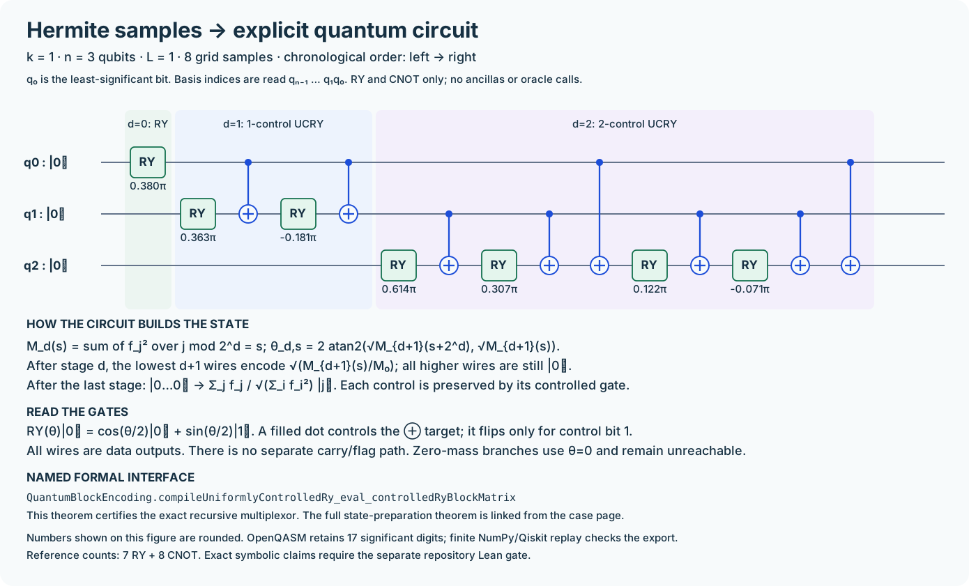
Open the chronological finite gate artifact
The original SVG is kept unchanged as replay evidence; its equations are baked vector text rather than MathJax. Use this page for the typeset mathematical reading.
Example circuit (OpenQASM 3)
OPENQASM 3.0;
include "stdgates.inc";
qubit[3] q;
ry(1.1952476818322655) q[0];
ry(1.1411899214842629) q[1];
cx q[0],q[1];
ry(-0.56983382256701454) q[1];
cx q[0],q[1];
ry(1.9282975397199893) q[2];
cx q[1],q[2];
ry(0.96514759743197598) q[2];
cx q[1],q[2];
cx q[0],q[2];
ry(0.38470990194757371) q[2];
cx q[1],q[2];
ry(-0.22293648255930965) q[2];
cx q[1],q[2];
cx q[0],q[2];
Accepted finite packet: OpenQASM 2 replay circuit
Accepted finite packet: OpenQASM 3 replay circuit
Sample positions and target amplitudes (CSV)
Saved mass-tree evidence required by independent replay (JSON)
Saved endpoint-jet evidence required by independent replay (JSON)
Finite replay results, backend versions and artifact hashes (JSON)
Register conventions and executable manifest (JSON)
Independent interpolation and saved-QASM replay
Independent interpolation and saved-QASM replay
#!/usr/bin/env python3
"""Replay saved artifacts using an independent rational Hermite interpolator.

No exporter functions are imported. Endpoint interpolation reconstructs the
target, while Qiskit parses and simulates the saved OpenQASM circuit.
"""
from __future__ import annotations

import argparse
import csv
from decimal import Decimal, localcontext
from fractions import Fraction
import hashlib
import json
import math
from pathlib import Path
import sys

import numpy as np


def interpolate(k: int) -> tuple[list[Fraction], list[Fraction]]:
    """Solve endpoint equations for P=exp(-1)*u+v by exact elimination."""
    if not isinstance(k, int) or not 0 <= k <= 30:
        raise ValueError("independent replay supports 0 <= k <= 30")
    size = 2*k+2
    matrix = []
    for endpoint in (0, 1):
        for order in range(k+1):
            row = [Fraction(math.factorial(i), math.factorial(i-order))*endpoint**(i-order)
                   if i >= order else Fraction(0) for i in range(size)]
            row.extend([Fraction(1), Fraction(0)] if endpoint == 0
                       else [Fraction(0), Fraction((-1)**order)])
            matrix.append(row)
    for col in range(size):
        pivot = next(i for i in range(col, size) if matrix[i][col])
        matrix[col], matrix[pivot] = matrix[pivot], matrix[col]
        divisor = matrix[col][col]
        matrix[col] = [x/divisor for x in matrix[col]]
        for row in range(size):
            if row != col and matrix[row][col]:
                factor = matrix[row][col]
                matrix[row] = [a-factor*b for a, b in zip(matrix[row], matrix[col])]
    return [row[size] for row in matrix], [row[size+1] for row in matrix]


def target_samples(k: int, n: int, length: float) -> tuple[np.ndarray, np.ndarray]:
    u, v = interpolate(k)
    points = -math.pi*length + 2*math.pi*length*np.arange(2**n)/2**n
    with localcontext() as context:
        context.prec = 100
        minus_one_exp = Decimal(-1).exp()
        coefficients = [minus_one_exp*Decimal(a.numerator)/Decimal(a.denominator)
                        + Decimal(b.numerator)/Decimal(b.denominator) for a, b in zip(u, v)]
        values = []
        for p in points:
            decimal_p = Decimal(str(p))
            if p <= -1:
                value = decimal_p.exp()
            elif p >= 0:
                value = (-decimal_p).exp()
            else:
                t = decimal_p+1
                value = Decimal(0)
                for coefficient in reversed(coefficients):
                    value = value*t+coefficient
            values.append(float(value))
    return points, np.asarray(values)


def verify(directory: Path) -> dict:
    from qiskit import qasm2, qasm3
    from qiskit.quantum_info import Statevector

    required = ["acceptance.json", "manifest.json", "circuit.qasm", "circuit.qasm2",
                "circuit.qasm3", "samples.csv", "mass-tree.json", "endpoint-jets.json"]
    for name in required:
        if not (directory/name).is_file():
            raise ValueError(f"required artifact is missing: {name}")
    acceptance = json.loads((directory/"acceptance.json").read_text(encoding="utf-8"))
    manifest = json.loads((directory/"manifest.json").read_text(encoding="utf-8"))
    if acceptance.get("accepted") is not True or acceptance.get("evidence_class") != "finite-executable-acceptance":
        raise ValueError("artifact does not claim completed executable acceptance")
    if acceptance.get("parameters") != manifest.get("parameters"):
        raise ValueError("manifest and acceptance parameters disagree")
    parameters = manifest["parameters"]
    k, n, length = parameters["k"], parameters["n"], parameters["L"]
    if not isinstance(n, int) or not 1 <= n <= 10 or not math.isfinite(length) or length <= 0:
        raise ValueError("invalid finite replay parameters")
    if n <= 5:
        required.append("circuit.svg")
    digests = acceptance.get("artifact_sha256", {})
    for name in required:
        if name == "acceptance.json":
            continue
        if not (directory/name).is_file():
            raise ValueError(f"required artifact is missing: {name}")
        actual = hashlib.sha256((directory/name).read_bytes()).hexdigest()
        if digests.get(name) != actual:
            raise ValueError(f"artifact hash mismatch: {name}")
    exporter = Path(__file__).with_name("export.py")
    if not exporter.is_file() or acceptance.get("exporter_sha256") != hashlib.sha256(exporter.read_bytes()).hexdigest():
        raise ValueError("exporter source changed after artifact acceptance")
    points, samples = target_samples(k, n, length)
    target = samples/np.linalg.norm(samples)
    with (directory/"samples.csv").open(encoding="utf-8", newline="") as stream:
        rows = list(csv.DictReader(stream))
    if len(rows) != 2**n:
        raise ValueError("wrong sample count")
    for j, row in enumerate(rows):
        if int(row["index"]) != j or row["basis_q_high_to_low"] != format(j, f"0{n}b"):
            raise ValueError("sample index or bit order mismatch")
    sample_error = max(float(np.max(np.abs(np.asarray([float(r[field]) for r in rows])-expected)))
                       for field, expected in (("p", points), ("f", samples), ("target_amplitude", target)))
    if sample_error > 1e-12:
        raise ValueError(f"independent endpoint interpolation disagrees with samples: {sample_error}")
    errors = {}
    for name, loader in (("circuit.qasm", qasm3.loads), ("circuit.qasm3", qasm3.loads), ("circuit.qasm2", qasm2.loads)):
        circuit = loader((directory/name).read_text(encoding="utf-8"))
        counts = circuit.count_ops()
        if circuit.num_qubits != n or set(counts) - {"ry", "cx"}:
            raise ValueError(f"unexpected wires or gates: {name}")
        if (counts.get("ry", 0), counts.get("cx", 0)) != (2**n-1, 2*(2**n-1-n)):
            raise ValueError(f"reference resource counts changed: {name}")
        state = np.asarray(Statevector.from_instruction(circuit).data)
        errors[name] = float(np.max(np.abs(state-target)))
    if max(errors.values()) > 1e-10:
        raise ValueError(f"independent QASM replay failed: {errors}")
    return {"passed": True, "evidence_class": "independent-finite-replay", "parameters": parameters,
            "target_method": "exact rational endpoint interpolation, evaluated at 100 decimal digits",
            "sample_max_error": sample_error, "qasm_max_amplitude_errors": errors,
            "checked_artifacts": required, "lean_certificate_claimed": False}


def main() -> int:
    parser = argparse.ArgumentParser(description=__doc__)
    parser.add_argument("--directory", type=Path, default=Path(__file__).resolve().parents[1])
    args = parser.parse_args()
    try:
        result = verify(args.directory)
    except (ValueError, KeyError, OSError, ImportError) as exc:
        print(f"Hermite independent replay failed: {exc}", file=sys.stderr)
        return 1
    print(json.dumps(result, indent=2, sort_keys=True, allow_nan=False))
    return 0


if __name__ == "__main__":
    raise SystemExit(main())
Mathematical target
The equation being studied
The samples themselves are amplitudes, not probabilities. The construction uses zero oracle calls and no postselection, and the bond register is clean at output. The exact-real quantum bound is certified separately from finite-bit implementation cost.
k- Number of endpoint derivatives matched; k=1 is the cubic splice.
n, N=2^n- Qubit count and sample count. q0 has weight 1.
L- Positive truncation parameter; grid interval [−πL,πL).
g_k(p_j)- Real amplitude before normalization, not a measurement probability.
Z_k- Sum of squared samples; normalization is proved from the actual input.
Circuit anatomy
How the candidate acts
These blocks show logical stages and register responsibilities. They do not pretend an unresolved logical oracle is already a primitive hardware gate.
Classical sample construction
Compute the Hermite coefficients and evaluate the two tails and the polynomial splice.
Mass reduction
Sum squared amplitudes over common low-bit prefixes. Each parent mass is the sum of its children.
Quantum preparation
Apply one uniformly controlled Ry layer per qubit, then compile every layer to Ry and CNOT.
Prepared register
The final amplitudes equal the normalized samples. Independent finite replay measures numerical rounding error.
Auditable evolution · certified milestones
Candidate and proof progression — how the certified construction changed
The project keeps the usual score order \((\text{gates},\text{depth},\text{auxiliary qubits},\text{oracle calls})\), but it does not compare unlike scopes as if they were one finite benchmark.
Scope. Displayed resource tuple is the preserved k=1, n_p=3, L=1 finite example.
Compute all sample masses, recursively split them by binary prefixes, and compile the resulting uniformly controlled rotations. This route is exact and pedagogically transparent, but it does not exploit the special function family when forming the preparation data.
Logical dataflow
QuantumBlockEncoding.HermiteStatePreparation.hermiteStatePreparation_complete
Scope. All-width exact-real quantum family for arbitrary natural k, n_p>=1 and positive L.
Keep the function in Bernstein / finite-state form, reinterpret that update rule as a bounded-bond tensor train, canonicalize the local maps and compile them to Ry/CNOT while cleaning the bond register.
Logical dataflow
QuantumBlockEncoding.ConstructiveHermitePreparation.prepare_spec
Reader workbench
Edit, preview, then copy
Change symbols, language, proof steps, or the grouped-register circuit locally in your browser. The preview is explanatory; the linked Lean declaration remains the certificate.
Mathematical construction
Proof steps
One step per line. Natural language and inline mathematics are both accepted.
Quantum circuit
Complete packet
Copy the reviewed construction and proof
The packet below is generated from the reviewed case record. The exact primitive authority is the linked Lean source and executable artifact.
Construction and circuit LaTeX
% Requires: \usepackage{quantikz}
\paragraph{Construction.}
\[
\lvert g_k\rangle_p=\frac{1}{\sqrt{Z_k}}\sum_{j=0}^{2^n-1}g_k(p_j)\lvert j\rangle,\quad Z_k=\sum_jg_k(p_j)^2,\quad p_j=-\pi L+\frac{2\pi Lj}{2^n}.
\]

% Hermite rotation tree
\begin{quantikz}[row sep=.45cm,column sep=.6cm]
\lstick{$q_0:\ket0$} & \gate{R_y} & \ctrl{1} & \ctrl{2} & \qw \\
\lstick{$q_1:\ket0$} & \qw & \gate{\mathrm{UCRY}_1} & \ctrl{1} & \qw \\
\lstick{$q_2:\ket0$} & \qw & \qw & \gate{\mathrm{UCRY}_2} & \rstick{$|g_k\rangle$} \qw
\end{quantikz}
English proof LaTeX
\paragraph{Proof.}
The exact target uses exp(p) to the left of −1, a degree-at-most 2k+1 Hermite polynomial on [−1,0], and exp(−p) to the right of 0. The real-valued samples, not their square roots, are normalized. The new Bernstein–MPS circuit has at most 48 n_p (2k+6)^3 Ry/CNOT instructions and the same upper bound on scheduled depth, with ceil(log2(2k+6)) clean bond qubits, zero oracle calls and no postselection. These are exact real-angle quantum bounds. Whole classical preprocessing and uniform finite-precision error remain open. The original exponential rotation tree and its finite downloadable packet are retained below as the reference.
\begin{enumerate}
  \item First construct the polynomial and its endpoint jets. Build the low-bit mass tree and apply its exact controlled rotations. The invariant says that a prefix carries the square root of its total remaining probability mass. The final layer resolves each requested amplitude.
\end{enumerate}
Each advertised certificate is the named Lean declaration linked on this page.
Lean declaration retrieval block
import QuantumBlockEncoding

#check QuantumBlockEncoding.HermitePolynomial.sourceInterpolant_degree
#check QuantumBlockEncoding.HermitePolynomial.sourceInterpolant_left_iteratedDeriv
#check QuantumBlockEncoding.HermitePolynomial.sourceInterpolant_right_iteratedDeriv
#check QuantumBlockEncoding.HermitePolynomial.coefficientPolynomial_eval
#check QuantumBlockEncoding.HermitePolynomial.sourceInterpolant_eval
#check QuantumBlockEncoding.HermitePolynomial.smoothInitial_pos
#check QuantumBlockEncoding.HermiteSmoothness.smoothInitial_contDiff
#check QuantumBlockEncoding.compileUniformlyControlledRy_eval_controlledRyBlockMatrix
#check QuantumBlockEncoding.HermiteStatePreparation.hermiteStatePreparation_complete
#check QuantumBlockEncoding.HermiteBoundaryInjection.hermiteKernel_eq_sample
#check QuantumBlockEncoding.HermiteFiniteNorm.localSampleNorm_eq_sampleNorm
#check QuantumBlockEncoding.ConstructiveHermitePreparation.prepare_spec
#check QuantumBlockEncoding.StoredTensorTrain.canonicalize_total_cost_le
#check QuantumBlockEncoding.StoredHermiteRawSource.raw_contract
#check QuantumBlockEncoding.StoredHermiteRawCost.raw_certified
#check QuantumBlockEncoding.PrimitiveRyPerturbation.eval_ry_distance
#check QuantumBlockEncoding.PrimitiveCircuitPerturbation.prepare_conditional_clm_distance_le
Show the complete Lean certificate list
Open this when you want to inspect every declaration linked to the case.
Proof authority
Named Lean certificates
These declarations, compiled by the current Lean gate, support the mathematical and resource claims above.
QuantumBlockEncoding.HermitePolynomial.sourceInterpolant_degreeQuantumBlockEncoding/HermitePolynomial.lean:325QuantumBlockEncoding.HermitePolynomial.sourceInterpolant_left_iteratedDerivQuantumBlockEncoding/HermitePolynomial.lean:346QuantumBlockEncoding.HermitePolynomial.sourceInterpolant_right_iteratedDerivQuantumBlockEncoding/HermitePolynomial.lean:351QuantumBlockEncoding.HermitePolynomial.coefficientPolynomial_evalQuantumBlockEncoding/HermitePolynomial.lean:289QuantumBlockEncoding.HermitePolynomial.sourceInterpolant_evalQuantumBlockEncoding/HermitePolynomial.lean:298QuantumBlockEncoding.HermitePolynomial.smoothInitial_posQuantumBlockEncoding/HermitePolynomial.lean:373QuantumBlockEncoding.HermiteSmoothness.smoothInitial_contDiffQuantumBlockEncoding/HermiteSmoothness.lean:145QuantumBlockEncoding.compileUniformlyControlledRy_eval_controlledRyBlockMatrixQuantumBlockEncoding/UniformlyControlledRy.lean:259QuantumBlockEncoding.HermiteStatePreparation.hermiteStatePreparation_completeQuantumBlockEncoding/HermiteStatePreparation.lean:96QuantumBlockEncoding.HermiteBoundaryInjection.hermiteKernel_eq_sampleQuantumBlockEncoding/HermiteBoundaryInjection.lean:1138QuantumBlockEncoding.HermiteFiniteNorm.localSampleNorm_eq_sampleNormQuantumBlockEncoding/HermiteFiniteNorm.lean:45QuantumBlockEncoding.ConstructiveHermitePreparation.prepare_specQuantumBlockEncoding/ConstructiveHermitePreparation.lean:72QuantumBlockEncoding.StoredTensorTrain.canonicalize_total_cost_leQuantumBlockEncoding/StoredTensorTrain.lean:232QuantumBlockEncoding.StoredHermiteRawSource.raw_contractQuantumBlockEncoding/StoredHermiteRawSource.lean:131QuantumBlockEncoding.StoredHermiteRawCost.raw_certifiedQuantumBlockEncoding/StoredHermiteRawCost.lean:218QuantumBlockEncoding.PrimitiveRyPerturbation.eval_ry_distanceQuantumBlockEncoding/PrimitiveRyPerturbation.lean:82QuantumBlockEncoding.PrimitiveCircuitPerturbation.prepare_conditional_clm_distance_leQuantumBlockEncoding/PrimitiveCircuitPerturbation.lean:121
Optional executable checks and outputs
Executable verification and exports
Checking and artifact selection are independent. A user may screen with Qiskit, OpenQASM round-trip, both, or neither, then request a different set of output files.
| Backend / artifact | Role | Status | Evidence |
|---|---|---|---|
| Internal canonical evaluator | Reference semantics for primitive canonical IR | passed | metrics manifest |
| Qiskit replay | Gate-by-gate numerical screening | passed | executable-exports/SP-HERMITE-001/qiskit/export.py |
| OpenQASM 3 round-trip | Strict serialization, import, and semantic replay | passed | QASM and report when generated |
| Lean certificate | Exact proof authority at the page's stated semantic tier | passed | 17 named root(s) |
Replays the actual Ry/CNOT gate list using independent NumPy and Qiskit evaluators and an OpenQASM round trip. Reports finite floating-point evidence, not a general exact certificate.
- Current runnable artifact
executable-exports/SP-HERMITE-001/qiskit/export.py- Command
python3 executable-exports/SP-HERMITE-001/qiskit/export.py --self-test
- Source
- Jin–Liu–Ma, arXiv:2403.19123v3, Section 4.3, Eqs. (4.31)–(4.32).
- Contributor
- ASPBE authors
- Current boundary
- For fixed k the new quantum gate/depth bound is linear in \(n_p\); k is not hidden as a constant when it varies. L is any positive real in Lean, but executable experiments accept positive rational L. Several stored preprocessing components have polynomial bounds in an explicit exact-real operation model; the composed full compiler and a uniform epsilon/bit-cost certificate remain open. Finite QASM replay is not a symbolic family certificate. PDE recovery, Fourier convergence, hardware synthesis and global optimality are outside this certificate. Arbitrary amplitude tables need not have a small bond dimension.